Functions to plot classes sir, mic and disk, with support for base R and ggplot2.
Especially the scale_*_mic() functions are relevant wrappers to plot MIC values for ggplot2. They allows custom MIC ranges and to plot intermediate log2 levels for missing MIC values.
Usage
scale_x_mic(keep_operators = "edges", mic_range = NULL, ...)

scale_y_mic(keep_operators = "edges", mic_range = NULL, ...)

scale_colour_mic(keep_operators = "edges", mic_range = NULL, ...)

scale_fill_mic(keep_operators = "edges", mic_range = NULL, ...)

scale_x_sir(colours_SIR = c(S = "#3CAEA3", SDD = "#8FD6C4", I = "#F6D55C", R
  = "#ED553B"), language = get_AMR_locale(),
  eucast_I = getOption("AMR_guideline", "EUCAST") == "EUCAST", ...)

scale_colour_sir(colours_SIR = c(S = "#3CAEA3", SDD = "#8FD6C4", I =
  "#F6D55C", R = "#ED553B"), language = get_AMR_locale(),
  eucast_I = getOption("AMR_guideline", "EUCAST") == "EUCAST", ...)

scale_fill_sir(colours_SIR = c(S = "#3CAEA3", SDD = "#8FD6C4", I = "#F6D55C",
  R = "#ED553B"), language = get_AMR_locale(),
  eucast_I = getOption("AMR_guideline", "EUCAST") == "EUCAST", ...)

# S3 method for class 'mic'
plot(x, mo = NULL, ab = NULL,
  guideline = getOption("AMR_guideline", "EUCAST"),
  main = deparse(substitute(x)), ylab = translate_AMR("Frequency", language
  = language),
  xlab = translate_AMR("Minimum Inhibitory Concentration (mg/L)", language =
  language), colours_SIR = c(S = "#3CAEA3", SDD = "#8FD6C4", I = "#F6D55C", R
  = "#ED553B"), language = get_AMR_locale(), expand = TRUE,
  include_PKPD = getOption("AMR_include_PKPD", TRUE),
  breakpoint_type = getOption("AMR_breakpoint_type", "human"), ...)

# S3 method for class 'mic'
autoplot(object, mo = NULL, ab = NULL,
  guideline = getOption("AMR_guideline", "EUCAST"),
  title = deparse(substitute(object)), ylab = translate_AMR("Frequency",
  language = language),
  xlab = translate_AMR("Minimum Inhibitory Concentration (mg/L)", language =
  language), colours_SIR = c(S = "#3CAEA3", SDD = "#8FD6C4", I = "#F6D55C", R
  = "#ED553B"), language = get_AMR_locale(), expand = TRUE,
  include_PKPD = getOption("AMR_include_PKPD", TRUE),
  breakpoint_type = getOption("AMR_breakpoint_type", "human"), ...)

# S3 method for class 'disk'
plot(x, main = deparse(substitute(x)),
  ylab = translate_AMR("Frequency", language = language),
  xlab = translate_AMR("Disk diffusion diameter (mm)", language = language),
  mo = NULL, ab = NULL, guideline = getOption("AMR_guideline", "EUCAST"),
  colours_SIR = c(S = "#3CAEA3", SDD = "#8FD6C4", I = "#F6D55C", R =
  "#ED553B"), language = get_AMR_locale(), expand = TRUE,
  include_PKPD = getOption("AMR_include_PKPD", TRUE),
  breakpoint_type = getOption("AMR_breakpoint_type", "human"), ...)

# S3 method for class 'disk'
autoplot(object, mo = NULL, ab = NULL,
  title = deparse(substitute(object)), ylab = translate_AMR("Frequency",
  language = language), xlab = translate_AMR("Disk diffusion diameter (mm)",
  language = language), guideline = getOption("AMR_guideline", "EUCAST"),
  colours_SIR = c(S = "#3CAEA3", SDD = "#8FD6C4", I = "#F6D55C", R =
  "#ED553B"), language = get_AMR_locale(), expand = TRUE,
  include_PKPD = getOption("AMR_include_PKPD", TRUE),
  breakpoint_type = getOption("AMR_breakpoint_type", "human"), ...)

# S3 method for class 'sir'
plot(x, ylab = translate_AMR("Percentage", language =
  language), xlab = translate_AMR("Antimicrobial Interpretation", language =
  language), main = deparse(substitute(x)), language = get_AMR_locale(),
  ...)

# S3 method for class 'sir'
autoplot(object, title = deparse(substitute(object)),
  xlab = translate_AMR("Antimicrobial Interpretation", language = language),
  ylab = translate_AMR("Frequency", language = language), colours_SIR = c(S
  = "#3CAEA3", SDD = "#8FD6C4", I = "#F6D55C", R = "#ED553B"),
  language = get_AMR_locale(), ...)

facet_sir(facet = c("interpretation", "antibiotic"), nrow = NULL)

scale_y_percent(breaks = function(x) seq(0, max(x, na.rm = TRUE), 0.1),
  limits = c(0, NA))

scale_sir_colours(..., aesthetics, colours_SIR = c(S = "#3CAEA3", SDD =
  "#8FD6C4", I = "#F6D55C", R = "#ED553B"))

theme_sir()

labels_sir_count(position = NULL, x = "antibiotic",
  translate_ab = "name", minimum = 30, language = get_AMR_locale(),
  combine_SI = TRUE, datalabels.size = 3, datalabels.colour = "grey15")
Arguments
- keep_operators
A character specifying how to handle operators (such as
>and<=) in the input. Accepts one of three values:"all"(orTRUE) to keep all operators,"none"(orFALSE) to remove all operators, or"edges"to keep operators only at both ends of the range.- mic_range
A manual range to rescale the MIC values (using
rescale_mic()), e.g.,mic_range = c(0.001, 32). UseNAto prevent rescaling on one side, e.g.,mic_range = c(NA, 32). Note: This rescales values but does not filter them - use the ggplot2limitsargument separately to exclude values from the plot.- ...
Arguments passed on to methods.
- colours_SIR
Colours to use for filling in the bars, must be a vector of three values (in the order S, I and R). The default colours are colour-blind friendly.
- language
Language to be used to translate 'Susceptible', 'Increased exposure'/'Intermediate' and 'Resistant' - the default is system language (see
get_AMR_locale()) and can be overwritten by setting the package optionAMR_locale, e.g.options(AMR_locale = "de"), see translate. Uselanguage = NULLto prevent translation.- eucast_I
A logical to indicate whether the 'I' must be interpreted as "Susceptible, under increased exposure". Will be
TRUEif the default AMR interpretation guideline is set to EUCAST (which is the default). WithFALSE, it will be interpreted as "Intermediate".- x, object
Values created with
as.mic(),as.disk()oras.sir()(or theirrandom_*variants, such asrandom_mic()).- mo
Any (vector of) text that can be coerced to a valid microorganism code with
as.mo().- ab
Any (vector of) text that can be coerced to a valid antimicrobial drug code with
as.ab().- guideline
Interpretation guideline to use - the default is the latest included EUCAST guideline, see Details.
- main, title
Title of the plot.
- xlab, ylab
Axis title.
- expand
A logical to indicate whether the range on the x axis should be expanded between the lowest and highest value. For MIC values, intermediate values will be factors of 2 starting from the highest MIC value. For disk diameters, the whole diameter range will be filled.
- include_PKPD
A logical to indicate that PK/PD clinical breakpoints must be applied as a last resort - the default is
TRUE. Can also be set with the package optionAMR_include_PKPD.- breakpoint_type
The type of breakpoints to use, either "ECOFF", "animal", or "human". ECOFF stands for Epidemiological Cut-Off values. The default is
"human", which can also be set with the package optionAMR_breakpoint_type. Ifhostis set to values of veterinary species, this will automatically be set to"animal".- facet
Variable to split plots by, either
"interpretation"(default) or"antibiotic"or a grouping variable.- nrow
(when using
facet) number of rows.- breaks
A numeric vector of positions.
- limits
A numeric vector of length two providing limits of the scale, use
NAto refer to the existing minimum or maximum.- aesthetics
Aesthetics to apply the colours to - the default is "fill" but can also be (a combination of) "alpha", "colour", "fill", "linetype", "shape" or "size".
- position
Position adjustment of bars, either
"fill","stack"or"dodge".- translate_ab
A column name of the antimicrobials data set to translate the antibiotic abbreviations to, using
ab_property().- minimum
The minimum allowed number of available (tested) isolates. Any isolate count lower than
minimumwill returnNAwith a warning. The default number of30isolates is advised by the Clinical and Laboratory Standards Institute (CLSI) as best practice, see Source.- combine_SI
A logical to indicate whether all values of S, SDD, and I must be merged into one, so the output only consists of S+SDD+I vs. R (susceptible vs. resistant) - the default is
TRUE.- datalabels.size
Size of the datalabels.
- datalabels.colour
Colour of the datalabels.
Value
The autoplot() functions return a ggplot model that is extendible with any ggplot2 function.
Details
The scale_*_mic() Functions
The functions scale_x_mic(), scale_y_mic(), scale_colour_mic(), and scale_fill_mic() functions allow to plot the mic class (MIC values) on a continuous, logarithmic scale. They also allow to rescale the MIC range with an 'inside' or 'outside' range if required, and retain the operators in MIC values (such as >=) if desired. Missing intermediate log2 levels will be plotted too.
The scale_*_sir() Functions
The functions scale_x_sir(), scale_colour_sir(), and scale_fill_sir() functions allow to plot the sir class in the right order (S < SDD < I < R < NI). At default, they translate the S/I/R values to an interpretative text ("Susceptible", "Resistant", etc.) in any of the 28 supported languages (use language = NULL to keep S/I/R). Also, except for scale_x_sir(), they set colour-blind friendly colours to the colour and fill aesthetics.
Additional ggplot2 Functions
This package contains more functions that extend the ggplot2 package, to help in visualising AMR data results. All these functions are internally used by ggplot_sir() too.
facet_sir()creates 2d plots (at default based on S/I/R) usingggplot2::facet_wrap().scale_y_percent()transforms the y axis to a 0 to 100% range usingggplot2::scale_y_continuous().scale_sir_colours()allows to set colours to any aesthetic, even forshapeorlinetype.theme_sir()is a ggplot2 theme with minimal distraction.labels_sir_count()print datalabels on the bars with percentage and number of isolates, usingggplot2::geom_text().
The interpretation of "I" will be named "Increased exposure" for all EUCAST guidelines since 2019, and will be named "Intermediate" in all other cases.
For interpreting MIC values as well as disk diffusion diameters, the default guideline is EUCAST 2025, unless the package option AMR_guideline is set. See as.sir() for more information.
Examples
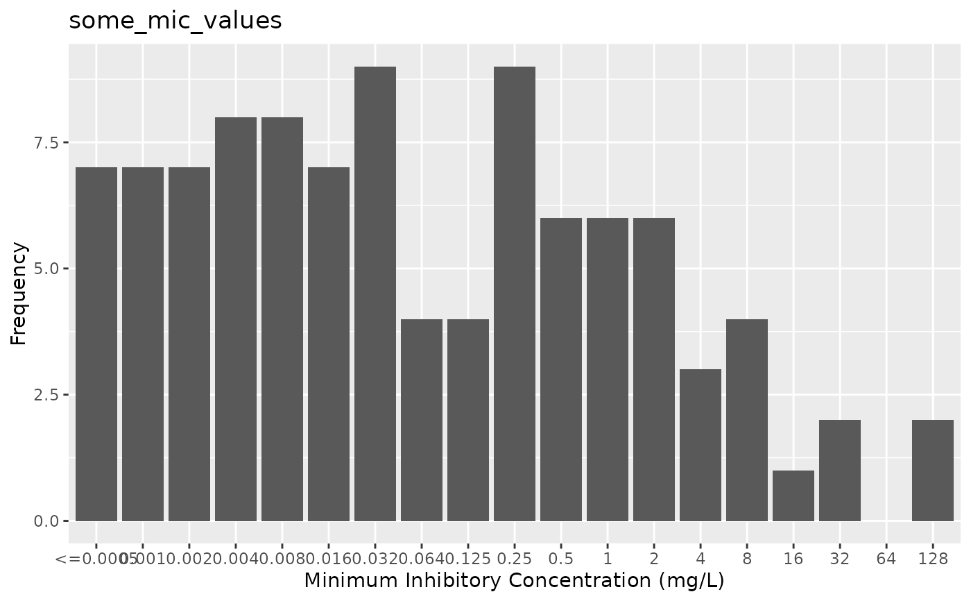
some_mic_values <- random_mic(size = 100)
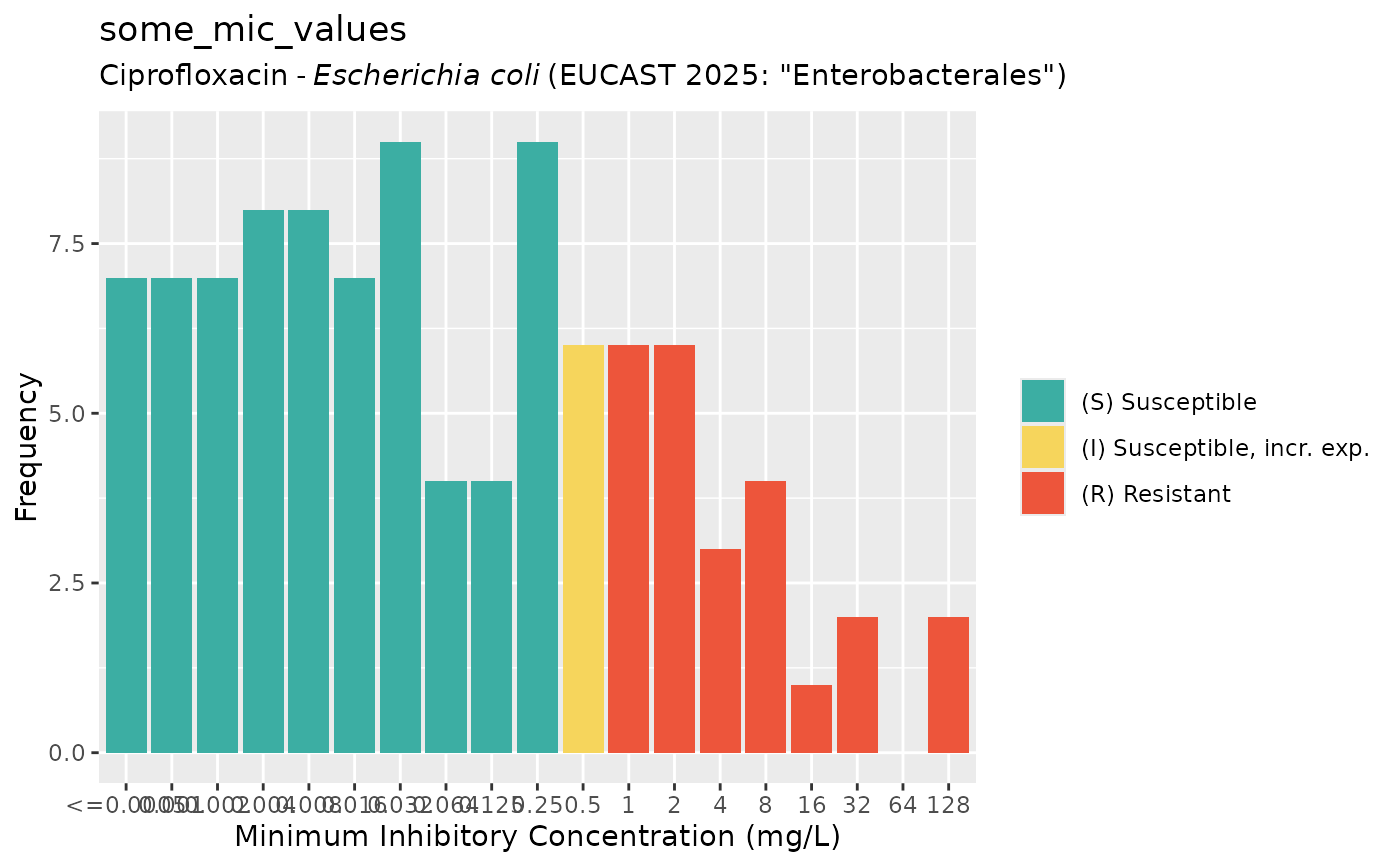
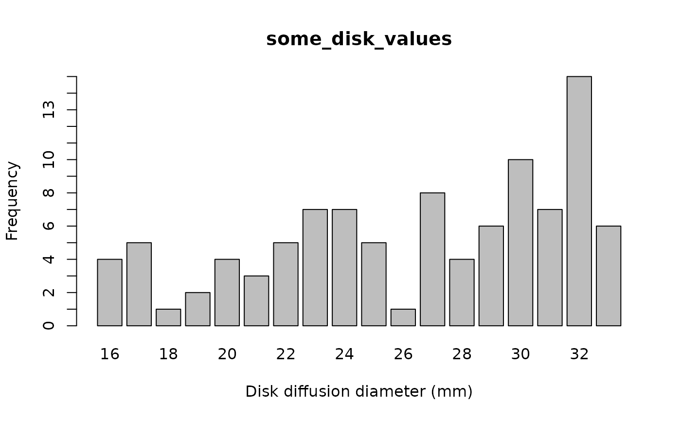
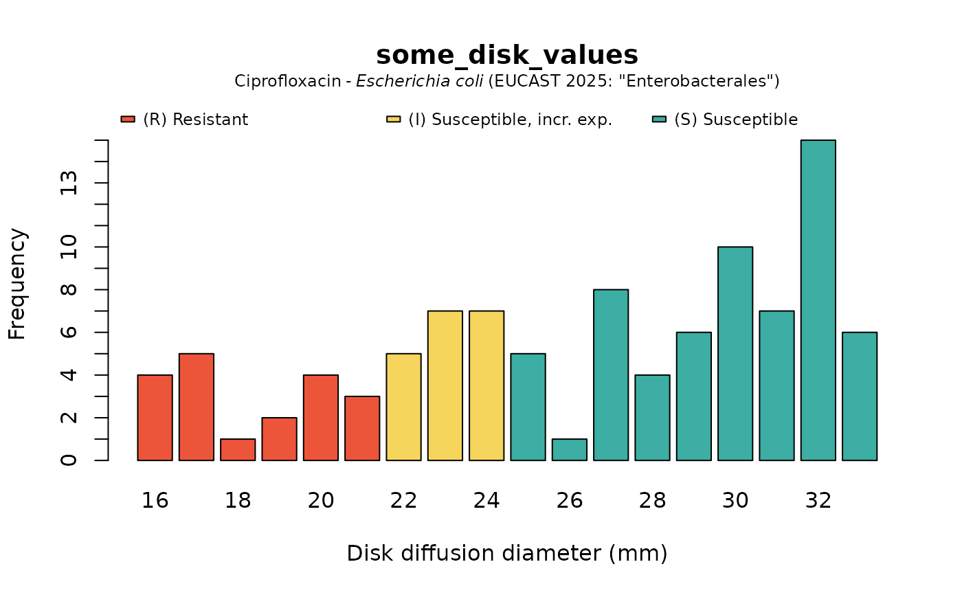
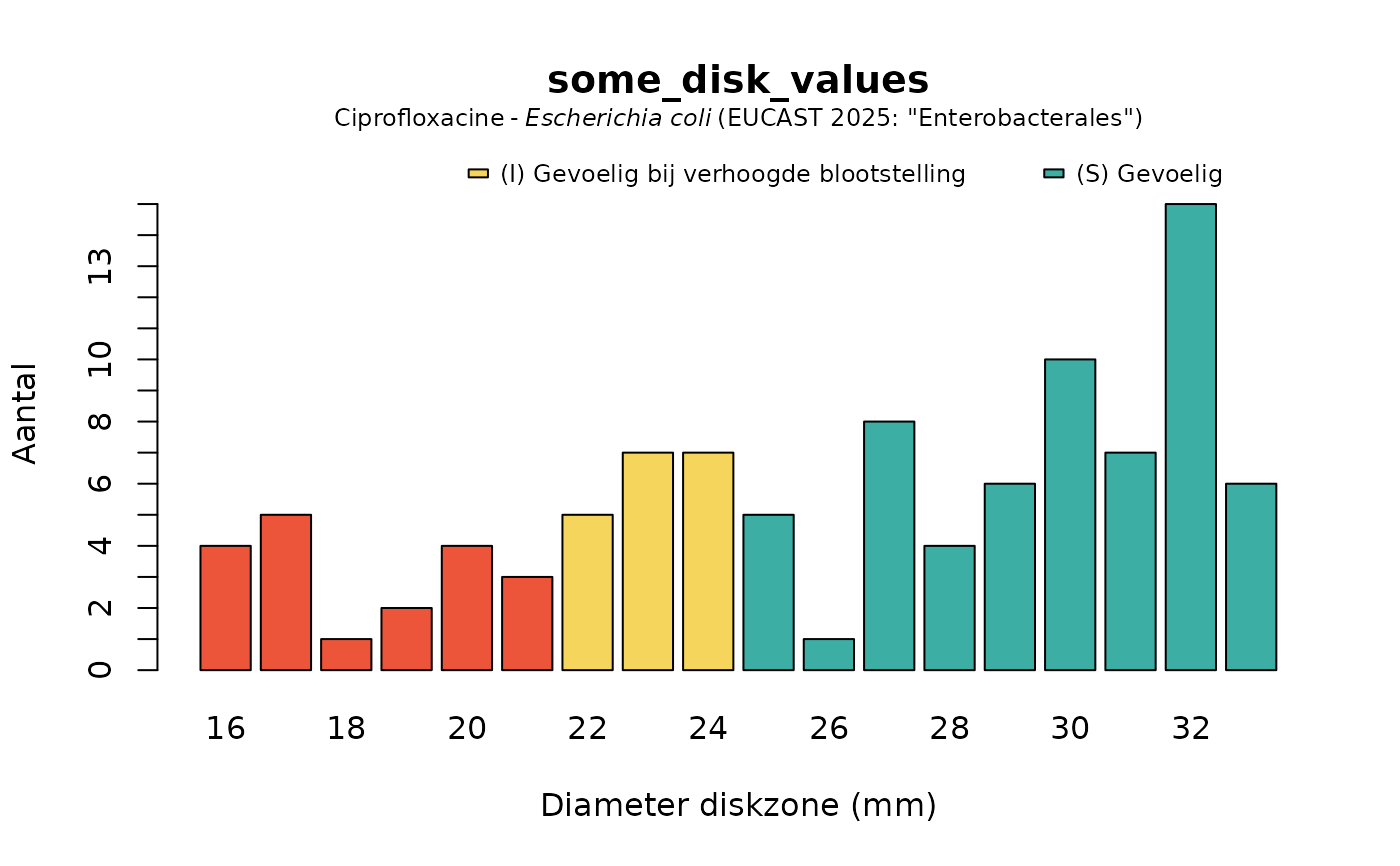
some_disk_values <- random_disk(size = 100, mo = "Escherichia coli", ab = "cipro")
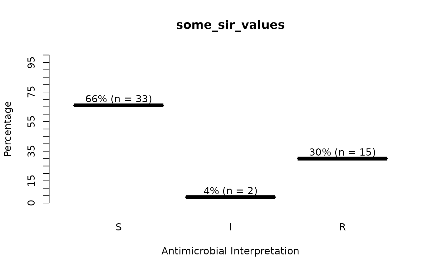
some_sir_values <- random_sir(50, prob_SIR = c(0.55, 0.05, 0.30))
# \donttest{
# Plotting using ggplot2's autoplot() for MIC, disk, and SIR -----------
if (require("ggplot2")) {
autoplot(some_mic_values)
}
 if (require("ggplot2")) {
# when providing the microorganism and antibiotic, colours will show interpretations:
autoplot(some_mic_values, mo = "Escherichia coli", ab = "cipro")
}
if (require("ggplot2")) {
# when providing the microorganism and antibiotic, colours will show interpretations:
autoplot(some_mic_values, mo = "Escherichia coli", ab = "cipro")
}
 if (require("ggplot2")) {
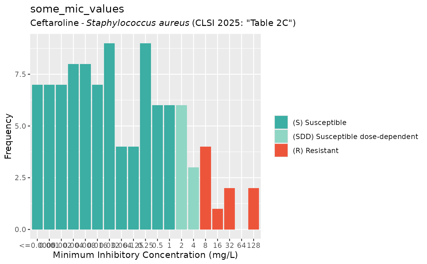
autoplot(some_mic_values, mo = "Staph aureus", ab = "Ceftaroline", guideline = "CLSI")
}
if (require("ggplot2")) {
autoplot(some_mic_values, mo = "Staph aureus", ab = "Ceftaroline", guideline = "CLSI")
}
 if (require("ggplot2")) {
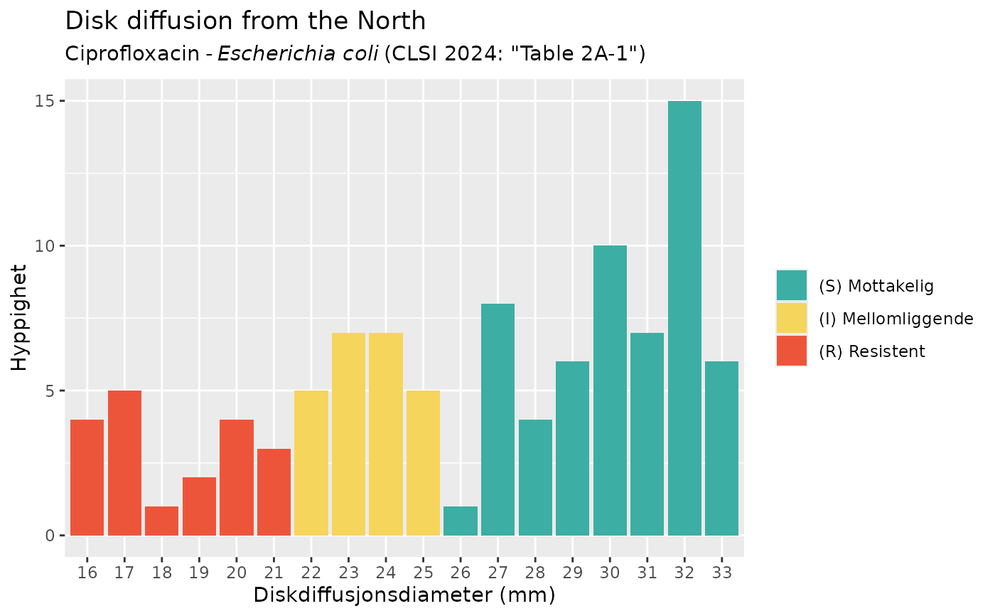
# support for 27 languages, various guidelines, and many options
autoplot(some_disk_values,
mo = "Escherichia coli", ab = "cipro",
guideline = "CLSI 2024", language = "no",
title = "Disk diffusion from the North"
)
}
if (require("ggplot2")) {
# support for 27 languages, various guidelines, and many options
autoplot(some_disk_values,
mo = "Escherichia coli", ab = "cipro",
guideline = "CLSI 2024", language = "no",
title = "Disk diffusion from the North"
)
}
 # Plotting using scale_x_mic() -----------------------------------------
if (require("ggplot2")) {
mic_plot <- ggplot(
data.frame(
mics = as.mic(c(0.25, "<=4", 4, 8, 32, ">=32")),
counts = c(1, 1, 2, 2, 3, 3)
),
aes(mics, counts)
) +
geom_col()
mic_plot +
labs(title = "without scale_x_mic()")
}
# Plotting using scale_x_mic() -----------------------------------------
if (require("ggplot2")) {
mic_plot <- ggplot(
data.frame(
mics = as.mic(c(0.25, "<=4", 4, 8, 32, ">=32")),
counts = c(1, 1, 2, 2, 3, 3)
),
aes(mics, counts)
) +
geom_col()
mic_plot +
labs(title = "without scale_x_mic()")
}
 if (require("ggplot2")) {
mic_plot +
scale_x_mic() +
labs(title = "with scale_x_mic()")
}
if (require("ggplot2")) {
mic_plot +
scale_x_mic() +
labs(title = "with scale_x_mic()")
}
 if (require("ggplot2")) {
mic_plot +
scale_x_mic(keep_operators = "all") +
labs(title = "with scale_x_mic() keeping all operators")
}
if (require("ggplot2")) {
mic_plot +
scale_x_mic(keep_operators = "all") +
labs(title = "with scale_x_mic() keeping all operators")
}
 if (require("ggplot2")) {
mic_plot +
scale_x_mic(mic_range = c(1, 16)) +
labs(title = "with scale_x_mic() using a manual 'within' range")
}
if (require("ggplot2")) {
mic_plot +
scale_x_mic(mic_range = c(1, 16)) +
labs(title = "with scale_x_mic() using a manual 'within' range")
}
 if (require("ggplot2")) {
mic_plot +
scale_x_mic(mic_range = c(0.032, 256)) +
labs(title = "with scale_x_mic() using a manual 'outside' range")
}
if (require("ggplot2")) {
mic_plot +
scale_x_mic(mic_range = c(0.032, 256)) +
labs(title = "with scale_x_mic() using a manual 'outside' range")
}
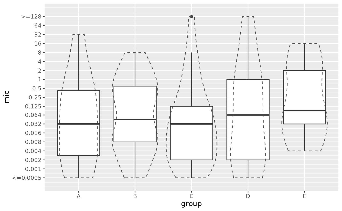
 # Plotting using scale_y_mic() -----------------------------------------
some_groups <- sample(LETTERS[1:5], 20, replace = TRUE)
if (require("ggplot2")) {
ggplot(
data.frame(
mic = some_mic_values,
group = some_groups
),
aes(group, mic)
) +
geom_boxplot() +
geom_violin(linetype = 2, colour = "grey30", fill = NA) +
scale_y_mic()
}
# Plotting using scale_y_mic() -----------------------------------------
some_groups <- sample(LETTERS[1:5], 20, replace = TRUE)
if (require("ggplot2")) {
ggplot(
data.frame(
mic = some_mic_values,
group = some_groups
),
aes(group, mic)
) +
geom_boxplot() +
geom_violin(linetype = 2, colour = "grey30", fill = NA) +
scale_y_mic()
}
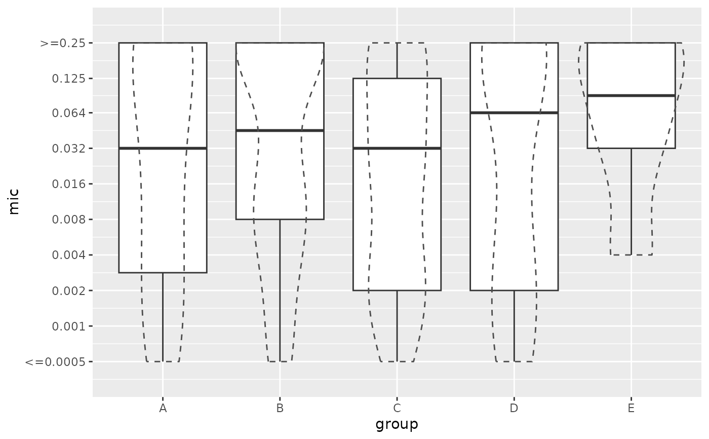
 if (require("ggplot2")) {
ggplot(
data.frame(
mic = some_mic_values,
group = some_groups
),
aes(group, mic)
) +
geom_boxplot() +
geom_violin(linetype = 2, colour = "grey30", fill = NA) +
scale_y_mic(mic_range = c(NA, 0.25))
}
if (require("ggplot2")) {
ggplot(
data.frame(
mic = some_mic_values,
group = some_groups
),
aes(group, mic)
) +
geom_boxplot() +
geom_violin(linetype = 2, colour = "grey30", fill = NA) +
scale_y_mic(mic_range = c(NA, 0.25))
}
 # Plotting using scale_x_sir() -----------------------------------------
if (require("ggplot2")) {
ggplot(
data.frame(
x = c("I", "R", "S"),
y = c(45, 323, 573)
),
aes(x, y)
) +
geom_col() +
scale_x_sir()
}
# Plotting using scale_x_sir() -----------------------------------------
if (require("ggplot2")) {
ggplot(
data.frame(
x = c("I", "R", "S"),
y = c(45, 323, 573)
),
aes(x, y)
) +
geom_col() +
scale_x_sir()
}
 # Plotting using scale_y_mic() and scale_colour_sir() ------------------
if (require("ggplot2")) {
plain <- ggplot(
data.frame(
mic = some_mic_values,
group = some_groups,
sir = as.sir(some_mic_values,
mo = "E. coli",
ab = "cipro"
)
),
aes(x = group, y = mic, colour = sir)
) +
theme_minimal() +
geom_boxplot(fill = NA, colour = "grey30") +
geom_jitter(width = 0.25)
plain
}
# Plotting using scale_y_mic() and scale_colour_sir() ------------------
if (require("ggplot2")) {
plain <- ggplot(
data.frame(
mic = some_mic_values,
group = some_groups,
sir = as.sir(some_mic_values,
mo = "E. coli",
ab = "cipro"
)
),
aes(x = group, y = mic, colour = sir)
) +
theme_minimal() +
geom_boxplot(fill = NA, colour = "grey30") +
geom_jitter(width = 0.25)
plain
}
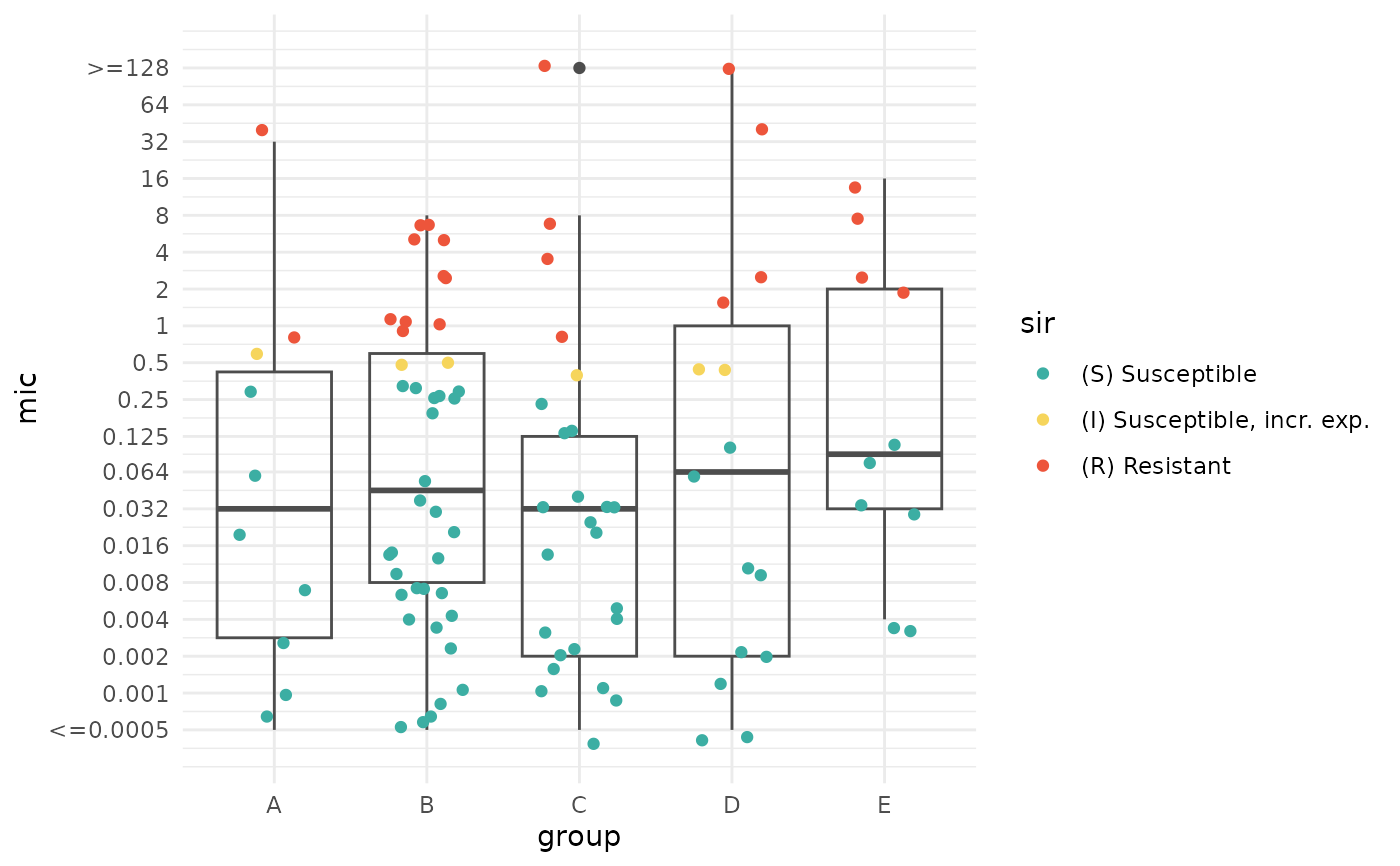
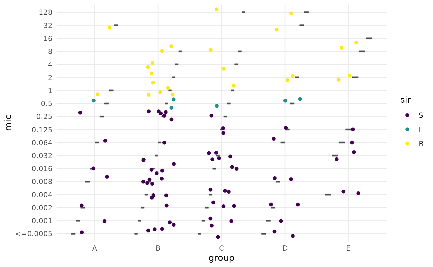 if (require("ggplot2")) {
# and now with our MIC and SIR scale functions:
plain +
scale_y_mic() +
scale_colour_sir()
}
if (require("ggplot2")) {
# and now with our MIC and SIR scale functions:
plain +
scale_y_mic() +
scale_colour_sir()
}
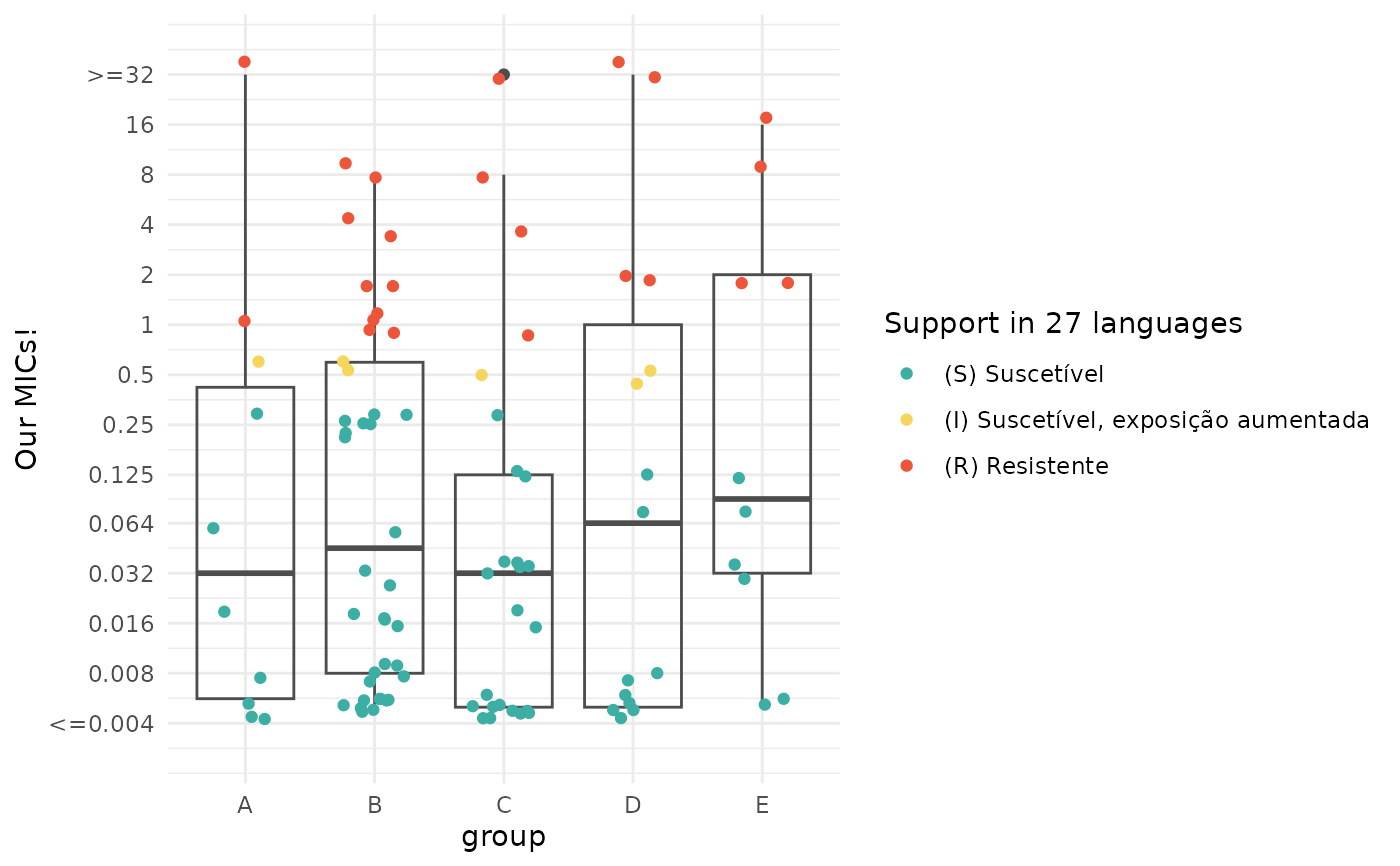
 if (require("ggplot2")) {
plain +
scale_y_mic(mic_range = c(0.005, 32), name = "Our MICs!") +
scale_colour_sir(
language = "pt",
name = "Support in 27 languages"
)
}
if (require("ggplot2")) {
plain +
scale_y_mic(mic_range = c(0.005, 32), name = "Our MICs!") +
scale_colour_sir(
language = "pt",
name = "Support in 27 languages"
)
}
 # }
# Plotting using base R's plot() ---------------------------------------
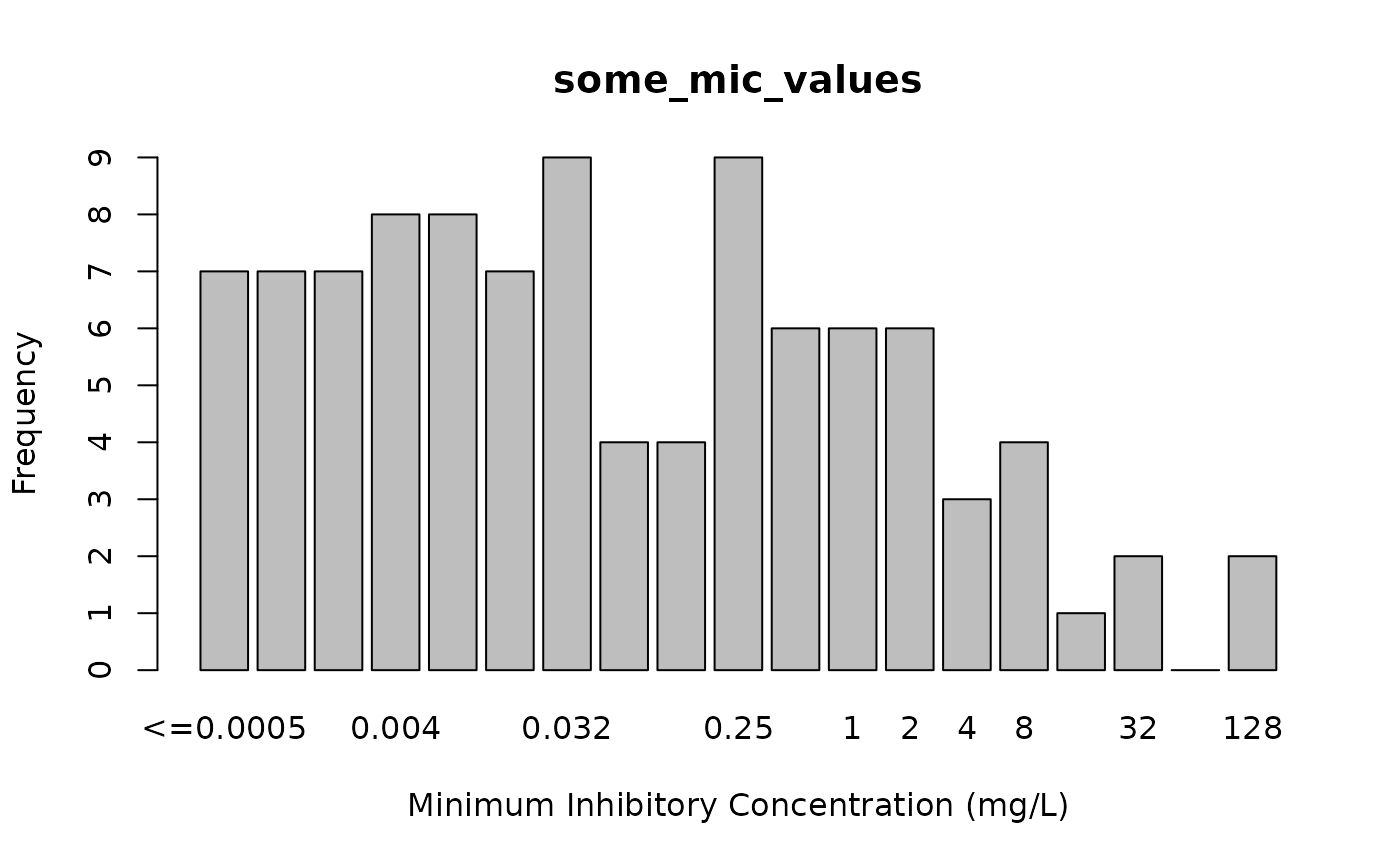
plot(some_mic_values)
# }
# Plotting using base R's plot() ---------------------------------------
plot(some_mic_values)
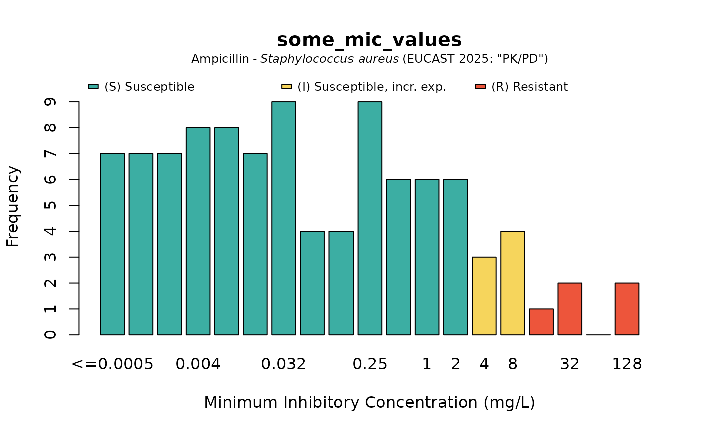
 # when providing the microorganism and antibiotic, colours will show interpretations:
plot(some_mic_values, mo = "S. aureus", ab = "ampicillin")
# when providing the microorganism and antibiotic, colours will show interpretations:
plot(some_mic_values, mo = "S. aureus", ab = "ampicillin")
 plot(some_disk_values)
 plot(some_disk_values, mo = "Escherichia coli", ab = "cipro")
 plot(some_disk_values, mo = "Escherichia coli", ab = "cipro", language = "nl")
 plot(some_sir_values)