How to conduct AMR analysis
Matthijs S. Berends
30 September 2019
AMR.RmdNote: values on this page will change with every website update since they are based on randomly created values and the page was written in R Markdown. However, the methodology remains unchanged. This page was generated on 30 September 2019.
Introduction
For this tutorial, we will create fake demonstration data to work with.
You can skip to Cleaning the data if you already have your own data ready. If you start your analysis, try to make the structure of your data generally look like this:
| date | patient_id | mo | AMX | CIP |
|---|---|---|---|---|
| 2019-09-30 | abcd | Escherichia coli | S | S |
| 2019-09-30 | abcd | Escherichia coli | S | R |
| 2019-09-30 | efgh | Escherichia coli | R | S |
Needed R packages
As with many uses in R, we need some additional packages for AMR analysis. Our package works closely together with the tidyverse packages dplyr and ggplot2 by Dr Hadley Wickham. The tidyverse tremendously improves the way we conduct data science - it allows for a very natural way of writing syntaxes and creating beautiful plots in R.
Our AMR package depends on these packages and even extends their use and functions.
Creation of data
We will create some fake example data to use for analysis. For antimicrobial resistance analysis, we need at least: a patient ID, name or code of a microorganism, a date and antimicrobial results (an antibiogram). It could also include a specimen type (e.g. to filter on blood or urine), the ward type (e.g. to filter on ICUs).
With additional columns (like a hospital name, the patients gender of even [well-defined] clinical properties) you can do a comparative analysis, as this tutorial will demonstrate too.
Patients
To start with patients, we need a unique list of patients.
The LETTERS object is available in R - it’s a vector with 26 characters: A to Z. The patients object we just created is now a vector of length 260, with values (patient IDs) varying from A1 to Z10. Now we we also set the gender of our patients, by putting the ID and the gender in a table:
The first 135 patient IDs are now male, the other 125 are female.
Dates
Let’s pretend that our data consists of blood cultures isolates from between 1 January 2010 and 1 January 2018.
This dates object now contains all days in our date range.
Other variables
For completeness, we can also add the hospital where the patients was admitted and we need to define valid antibmicrobial results for our randomisation:
Put everything together
Using the sample() function, we can randomly select items from all objects we defined earlier. To let our fake data reflect reality a bit, we will also approximately define the probabilities of bacteria and the antibiotic results with the prob parameter.
sample_size <- 20000
data <- data.frame(date = sample(dates, size = sample_size, replace = TRUE),
                   patient_id = sample(patients, size = sample_size, replace = TRUE),
                   hospital = sample(hospitals, size = sample_size, replace = TRUE,
                                     prob = c(0.30, 0.35, 0.15, 0.20)),
                   bacteria = sample(bacteria, size = sample_size, replace = TRUE,
                                     prob = c(0.50, 0.25, 0.15, 0.10)),
                   AMX = sample(ab_interpretations, size = sample_size, replace = TRUE,
                                 prob = c(0.60, 0.05, 0.35)),
                   AMC = sample(ab_interpretations, size = sample_size, replace = TRUE,
                                 prob = c(0.75, 0.10, 0.15)),
                   CIP = sample(ab_interpretations, size = sample_size, replace = TRUE,
                                 prob = c(0.80, 0.00, 0.20)),
                   GEN = sample(ab_interpretations, size = sample_size, replace = TRUE,
                                 prob = c(0.92, 0.00, 0.08)))
Using the left_join() function from the dplyr package, we can ‘map’ the gender to the patient ID using the patients_table object we created earlier:
The resulting data set contains 20,000 blood culture isolates. With the head() function we can preview the first 6 values of this data set:
| date | patient_id | hospital | bacteria | AMX | AMC | CIP | GEN | gender |
|---|---|---|---|---|---|---|---|---|
| 2016-02-07 | I4 | Hospital B | Escherichia coli | S | S | S | S | M |
| 2015-09-17 | V3 | Hospital B | Streptococcus pneumoniae | R | S | S | S | F |
| 2015-02-01 | K5 | Hospital B | Escherichia coli | S | S | S | S | M |
| 2010-03-05 | X1 | Hospital C | Klebsiella pneumoniae | R | R | S | S | F |
| 2012-01-13 | V5 | Hospital B | Staphylococcus aureus | S | S | S | S | F |
| 2014-11-13 | C4 | Hospital B | Escherichia coli | S | S | S | S | M |
Now, let’s start the cleaning and the analysis!
Cleaning the data
We also created a package dedicated to data cleaning and checking, called the clean package. It gets automatically installed with the AMR package, so we only have to load it:
Use the frequency table function freq() from this clean package to look specifically for unique values in any variable. For example, for the gender variable:
# Frequency table
#
# Class:   factor (numeric)
# Length:  20,000 (of which NA: 0 = 0%)
# Levels:  2: F, M
# Unique:  2
#
#      Item     Count   Percent   Cum. Count   Cum. Percent
# ---  -----  -------  --------  -----------  -------------
# 1    M       10,446    52.23%       10,446         52.23%
# 2    F        9,554    47.77%       20,000        100.00%
So, we can draw at least two conclusions immediately. From a data scientists perspective, the data looks clean: only values M and F. From a researchers perspective: there are slightly more men. Nothing we didn’t already know.
The data is already quite clean, but we still need to transform some variables. The bacteria column now consists of text, and we want to add more variables based on microbial IDs later on. So, we will transform this column to valid IDs. The mutate() function of the dplyr package makes this really easy:
We also want to transform the antibiotics, because in real life data we don’t know if they are really clean. The as.rsi() function ensures reliability and reproducibility in these kind of variables. The mutate_at() will run the as.rsi() function on defined variables:
Finally, we will apply EUCAST rules on our antimicrobial results. In Europe, most medical microbiological laboratories already apply these rules. Our package features their latest insights on intrinsic resistance and exceptional phenotypes. Moreover, the eucast_rules() function can also apply additional rules, like forcing
Because the amoxicillin (column AMX) and amoxicillin/clavulanic acid (column AMC) in our data were generated randomly, some rows will undoubtedly contain AMX = S and AMC = R, which is technically impossible. The eucast_rules() fixes this:
data <- eucast_rules(data, col_mo = "bacteria")
#
# Rules by the European Committee on Antimicrobial Susceptibility Testing (EUCAST)
# http://eucast.org/
#
# EUCAST Clinical Breakpoints (v9.0, 2019)
# Aerococcus sanguinicola (no changes)
# Aerococcus urinae (no changes)
# Anaerobic Gram-negatives (no changes)
# Anaerobic Gram-positives (no changes)
# Campylobacter coli (no changes)
# Campylobacter jejuni (no changes)
# Enterobacteriales (Order) (no changes)
# Enterococcus (no changes)
# Haemophilus influenzae (no changes)
# Kingella kingae (no changes)
# Moraxella catarrhalis (no changes)
# Pasteurella multocida (no changes)
# Staphylococcus (no changes)
# Streptococcus groups A, B, C, G (no changes)
# Streptococcus pneumoniae (1,448 values changed)
# Viridans group streptococci (no changes)
#
# EUCAST Expert Rules, Intrinsic Resistance and Exceptional Phenotypes (v3.1, 2016)
# Table 01: Intrinsic resistance in Enterobacteriaceae (1,335 values changed)
# Table 02: Intrinsic resistance in non-fermentative Gram-negative bacteria (no changes)
# Table 03: Intrinsic resistance in other Gram-negative bacteria (no changes)
# Table 04: Intrinsic resistance in Gram-positive bacteria (2,751 values changed)
# Table 08: Interpretive rules for B-lactam agents and Gram-positive cocci (no changes)
# Table 09: Interpretive rules for B-lactam agents and Gram-negative rods (no changes)
# Table 11: Interpretive rules for macrolides, lincosamides, and streptogramins (no changes)
# Table 12: Interpretive rules for aminoglycosides (no changes)
# Table 13: Interpretive rules for quinolones (no changes)
#
# Other rules
# Non-EUCAST: amoxicillin/clav acid = S where ampicillin = S (2,259 values changed)
# Non-EUCAST: ampicillin = R where amoxicillin/clav acid = R (125 values changed)
# Non-EUCAST: piperacillin = R where piperacillin/tazobactam = R (no changes)
# Non-EUCAST: piperacillin/tazobactam = S where piperacillin = S (no changes)
# Non-EUCAST: trimethoprim = R where trimethoprim/sulfa = R (no changes)
# Non-EUCAST: trimethoprim/sulfa = S where trimethoprim = S (no changes)
#
# --------------------------------------------------------------------------
# EUCAST rules affected 6,609 out of 20,000 rows, making a total of 7,918 edits
# => added 0 test results
#
# => changed 7,918 test results
#    - 101 test results changed from S to I
#    - 4,771 test results changed from S to R
#    - 1,065 test results changed from I to S
#    - 321 test results changed from I to R
#    - 1,636 test results changed from R to S
#    - 24 test results changed from R to I
# --------------------------------------------------------------------------
#
# Use eucast_rules(..., verbose = TRUE) (on your original data) to get a data.frame with all specified edits instead.
Adding new variables
Now that we have the microbial ID, we can add some taxonomic properties:
data <- data %>%
  mutate(gramstain = mo_gramstain(bacteria),
         genus = mo_genus(bacteria),
         species = mo_species(bacteria))
First isolates
We also need to know which isolates we can actually use for analysis.
To conduct an analysis of antimicrobial resistance, you must only include the first isolate of every patient per episode (Hindler et al., Clin Infect Dis. 2007). If you would not do this, you could easily get an overestimate or underestimate of the resistance of an antibiotic. Imagine that a patient was admitted with an MRSA and that it was found in 5 different blood cultures the following weeks (yes, some countries like the Netherlands have these blood drawing policies). The resistance percentage of oxacillin of all isolates would be overestimated, because you included this MRSA more than once. It would clearly be selection bias.
The Clinical and Laboratory Standards Institute (CLSI) appoints this as follows:
(…) When preparing a cumulative antibiogram to guide clinical decisions about empirical antimicrobial therapy of initial infections, only the first isolate of a given species per patient, per analysis period (eg, one year) should be included, irrespective of body site, antimicrobial susceptibility profile, or other phenotypical characteristics (eg, biotype). The first isolate is easily identified, and cumulative antimicrobial susceptibility test data prepared using the first isolate are generally comparable to cumulative antimicrobial susceptibility test data calculated by other methods, providing duplicate isolates are excluded.
M39-A4 Analysis and Presentation of Cumulative Antimicrobial Susceptibility Test Data, 4th Edition. CLSI, 2014. Chapter 6.4
This AMR package includes this methodology with the first_isolate() function. It adopts the episode of a year (can be changed by user) and it starts counting days after every selected isolate. This new variable can easily be added to our data:
data <- data %>%
  mutate(first = first_isolate(.))
# NOTE: Using column `bacteria` as input for `col_mo`.
# NOTE: Using column `date` as input for `col_date`.
# NOTE: Using column `patient_id` as input for `col_patient_id`.
# => Found 5,685 first isolates (28.4% of total)
So only 28.4% is suitable for resistance analysis! We can now filter on it with the filter() function, also from the dplyr package:
For future use, the above two syntaxes can be shortened with the filter_first_isolate() function:
First weighted isolates
We made a slight twist to the CLSI algorithm, to take into account the antimicrobial susceptibility profile. Have a look at all isolates of patient K5, sorted on date:
| isolate | date | patient_id | bacteria | AMX | AMC | CIP | GEN | first |
|---|---|---|---|---|---|---|---|---|
| 1 | 2010-04-28 | K5 | B_ESCHR_COLI | S | S | R | S | TRUE |
| 2 | 2010-06-18 | K5 | B_ESCHR_COLI | S | S | S | S | FALSE |
| 3 | 2010-10-15 | K5 | B_ESCHR_COLI | R | S | S | S | FALSE |
| 4 | 2010-12-16 | K5 | B_ESCHR_COLI | S | S | S | S | FALSE |
| 5 | 2011-01-17 | K5 | B_ESCHR_COLI | S | S | S | S | FALSE |
| 6 | 2011-06-30 | K5 | B_ESCHR_COLI | S | S | S | S | TRUE |
| 7 | 2011-08-11 | K5 | B_ESCHR_COLI | R | S | S | S | FALSE |
| 8 | 2011-10-18 | K5 | B_ESCHR_COLI | R | R | S | S | FALSE |
| 9 | 2012-04-24 | K5 | B_ESCHR_COLI | I | S | S | R | FALSE |
| 10 | 2012-10-30 | K5 | B_ESCHR_COLI | R | S | S | S | TRUE |
Only 3 isolates are marked as ‘first’ according to CLSI guideline. But when reviewing the antibiogram, it is obvious that some isolates are absolutely different strains and should be included too. This is why we weigh isolates, based on their antibiogram. The key_antibiotics() function adds a vector with 18 key antibiotics: 6 broad spectrum ones, 6 small spectrum for Gram negatives and 6 small spectrum for Gram positives. These can be defined by the user.
If a column exists with a name like ‘key(…)ab’ the first_isolate() function will automatically use it and determine the first weighted isolates. Mind the NOTEs in below output:
data <- data %>%
  mutate(keyab = key_antibiotics(.)) %>%
  mutate(first_weighted = first_isolate(.))
# NOTE: Using column `bacteria` as input for `col_mo`.
# NOTE: Using column `bacteria` as input for `col_mo`.
# NOTE: Using column `date` as input for `col_date`.
# NOTE: Using column `patient_id` as input for `col_patient_id`.
# NOTE: Using column `keyab` as input for `col_keyantibiotics`. Use col_keyantibiotics = FALSE to prevent this.
# [Criterion] Inclusion based on key antibiotics, ignoring I.
# => Found 15,102 first weighted isolates (75.5% of total)| isolate | date | patient_id | bacteria | AMX | AMC | CIP | GEN | first | first_weighted |
|---|---|---|---|---|---|---|---|---|---|
| 1 | 2010-04-28 | K5 | B_ESCHR_COLI | S | S | R | S | TRUE | TRUE |
| 2 | 2010-06-18 | K5 | B_ESCHR_COLI | S | S | S | S | FALSE | TRUE |
| 3 | 2010-10-15 | K5 | B_ESCHR_COLI | R | S | S | S | FALSE | TRUE |
| 4 | 2010-12-16 | K5 | B_ESCHR_COLI | S | S | S | S | FALSE | TRUE |
| 5 | 2011-01-17 | K5 | B_ESCHR_COLI | S | S | S | S | FALSE | FALSE |
| 6 | 2011-06-30 | K5 | B_ESCHR_COLI | S | S | S | S | TRUE | TRUE |
| 7 | 2011-08-11 | K5 | B_ESCHR_COLI | R | S | S | S | FALSE | TRUE |
| 8 | 2011-10-18 | K5 | B_ESCHR_COLI | R | R | S | S | FALSE | TRUE |
| 9 | 2012-04-24 | K5 | B_ESCHR_COLI | I | S | S | R | FALSE | TRUE |
| 10 | 2012-10-30 | K5 | B_ESCHR_COLI | R | S | S | S | TRUE | TRUE |
Instead of 3, now 9 isolates are flagged. In total, 75.5% of all isolates are marked ‘first weighted’ - 47.1% more than when using the CLSI guideline. In real life, this novel algorithm will yield 5-10% more isolates than the classic CLSI guideline.
As with filter_first_isolate(), there’s a shortcut for this new algorithm too:
So we end up with 15,102 isolates for analysis.
We can remove unneeded columns:
Now our data looks like:
| date | patient_id | hospital | bacteria | AMX | AMC | CIP | GEN | gender | gramstain | genus | species | first_weighted | |
|---|---|---|---|---|---|---|---|---|---|---|---|---|---|
| 1 | 2016-02-07 | I4 | Hospital B | B_ESCHR_COLI | S | S | S | S | M | Gram-negative | Escherichia | coli | TRUE |
| 2 | 2015-09-17 | V3 | Hospital B | B_STRPT_PNMN | R | R | S | R | F | Gram-positive | Streptococcus | pneumoniae | TRUE |
| 3 | 2015-02-01 | K5 | Hospital B | B_ESCHR_COLI | S | S | S | S | M | Gram-negative | Escherichia | coli | TRUE |
| 4 | 2010-03-05 | X1 | Hospital C | B_KLBSL_PNMN | R | R | S | S | F | Gram-negative | Klebsiella | pneumoniae | TRUE |
| 7 | 2016-04-24 | I9 | Hospital A | B_STPHY_AURS | R | S | S | S | M | Gram-positive | Staphylococcus | aureus | TRUE |
| 9 | 2015-09-18 | O7 | Hospital A | B_ESCHR_COLI | R | S | S | S | F | Gram-negative | Escherichia | coli | TRUE |
Time for the analysis!
Analysing the data
You might want to start by getting an idea of how the data is distributed. It’s an important start, because it also decides how you will continue your analysis. Although this package contains a convenient function to make frequency tables, exploratory data analysis (EDA) is not the primary scope of this package. Use a package like DataExplorer for that, or read the free online book Exploratory Data Analysis with R by Roger D. Peng.
Dispersion of species
To just get an idea how the species are distributed, create a frequency table with our freq() function. We created the genus and species column earlier based on the microbial ID. With paste(), we can concatenate them together.
The freq() function can be used like the base R language was intended:
Or can be used like the dplyr way, which is easier readable:
Frequency table
Class: character
Length: 15,102 (of which NA: 0 = 0%)
Unique: 4
Shortest: 16
Longest: 24
| Item | Count | Percent | Cum. Count | Cum. Percent | |
|---|---|---|---|---|---|
| 1 | Escherichia coli | 7,408 | 49.05% | 7,408 | 49.05% |
| 2 | Staphylococcus aureus | 3,747 | 24.81% | 11,155 | 73.86% |
| 3 | Streptococcus pneumoniae | 2,341 | 15.50% | 13,496 | 89.37% |
| 4 | Klebsiella pneumoniae | 1,606 | 10.63% | 15,102 | 100.00% |
Resistance percentages
The functions portion_S(), portion_SI(), portion_I(), portion_IR() and portion_R() can be used to determine the portion of a specific antimicrobial outcome. As per the EUCAST guideline of 2019, we calculate resistance as the portion of R (portion_R()) and susceptibility as the portion of S and I (portion_SI()). These functions can be used on their own:
Or can be used in conjuction with group_by() and summarise(), both from the dplyr package:
| hospital | amoxicillin |
|---|---|
| Hospital A | 0.4653354 |
| Hospital B | 0.4673178 |
| Hospital C | 0.4720576 |
| Hospital D | 0.4613045 |
Of course it would be very convenient to know the number of isolates responsible for the percentages. For that purpose the n_rsi() can be used, which works exactly like n_distinct() from the dplyr package. It counts all isolates available for every group (i.e. values S, I or R):
| hospital | amoxicillin | available |
|---|---|---|
| Hospital A | 0.4653354 | 4457 |
| Hospital B | 0.4673178 | 5324 |
| Hospital C | 0.4720576 | 2362 |
| Hospital D | 0.4613045 | 2959 |
These functions can also be used to get the portion of multiple antibiotics, to calculate empiric susceptibility of combination therapies very easily:
data_1st %>%
  group_by(genus) %>%
  summarise(amoxiclav = portion_SI(AMC),
            gentamicin = portion_SI(GEN),
amoxiclav_genta = portion_SI(AMC, GEN))| genus | amoxiclav | gentamicin | amoxiclav_genta |
|---|---|---|---|
| Escherichia | 0.9226512 | 0.8964633 | 0.9943305 |
| Klebsiella | 0.8281445 | 0.8953923 | 0.9856787 |
| Staphylococcus | 0.9236723 | 0.9196691 | 0.9954630 |
| Streptococcus | 0.6253738 | 0.0000000 | 0.6253738 |
To make a transition to the next part, let’s see how this difference could be plotted:
data_1st %>%
  group_by(genus) %>%
  summarise("1. Amoxi/clav" = portion_SI(AMC),
            "2. Gentamicin" = portion_SI(GEN),
            "3. Amoxi/clav + genta" = portion_SI(AMC, GEN)) %>%
  tidyr::gather("antibiotic", "S", -genus) %>%
  ggplot(aes(x = genus,
             y = S,
             fill = antibiotic)) +
  geom_col(position = "dodge2")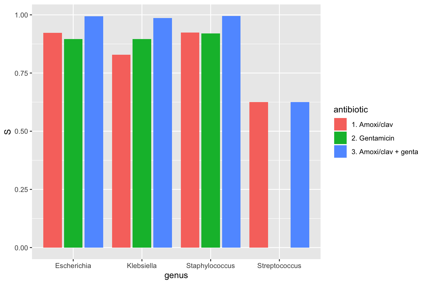
Plots
To show results in plots, most R users would nowadays use the ggplot2 package. This package lets you create plots in layers. You can read more about it on their website. A quick example would look like these syntaxes:
ggplot(data = a_data_set,
       mapping = aes(x = year,
                     y = value)) +
  geom_col() +
  labs(title = "A title",
       subtitle = "A subtitle",
       x = "My X axis",
       y = "My Y axis")

# or as short as:
ggplot(a_data_set) +
  geom_bar(aes(year))
The AMR package contains functions to extend this ggplot2 package, for example geom_rsi(). It automatically transforms data with count_df() or portion_df() and show results in stacked bars. Its simplest and shortest example:
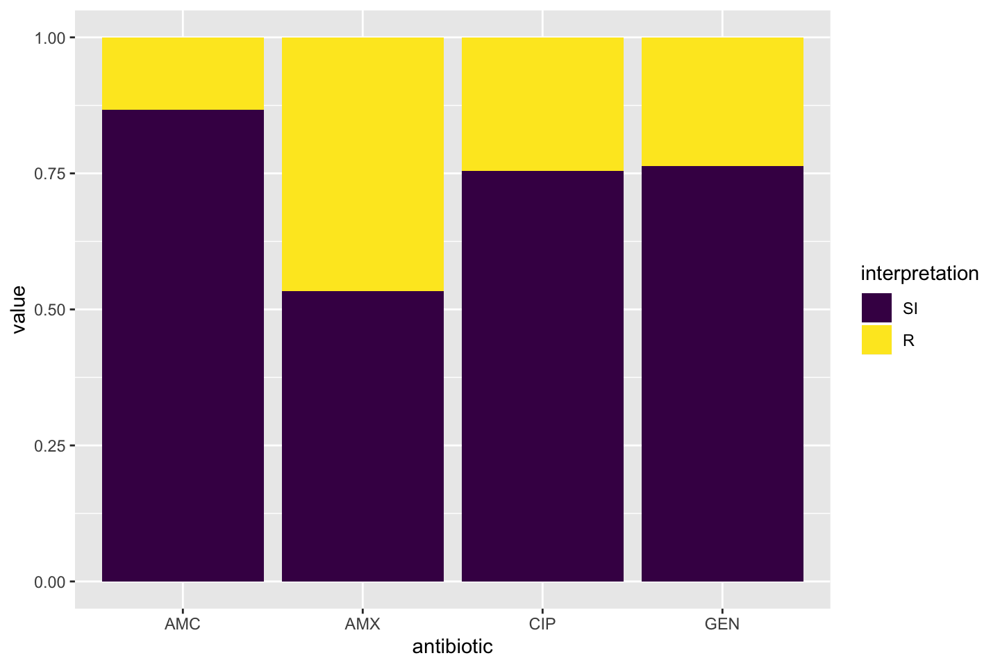
Omit the translate_ab = FALSE to have the antibiotic codes (AMX, AMC, CIP, GEN) translated to official WHO names (amoxicillin, amoxicillin/clavulanic acid, ciprofloxacin, gentamicin).
If we group on e.g. the genus column and add some additional functions from our package, we can create this:
# group the data on `genus`
ggplot(data_1st %>% group_by(genus)) +
  # create bars with genus on x axis
  # it looks for variables with class `rsi`,
  # of which we have 4 (earlier created with `as.rsi`)
  geom_rsi(x = "genus") +
  # split plots on antibiotic
  facet_rsi(facet = "antibiotic") +
  # make R red, I yellow and S green
  scale_rsi_colours() +
  # show percentages on y axis
  scale_y_percent(breaks = 0:4 * 25) +
  # turn 90 degrees, to make it bars instead of columns
  coord_flip() +
  # add labels
  labs(title = "Resistance per genus and antibiotic",
       subtitle = "(this is fake data)") +
  # and print genus in italic to follow our convention
  # (is now y axis because we turned the plot)
  theme(axis.text.y = element_text(face = "italic"))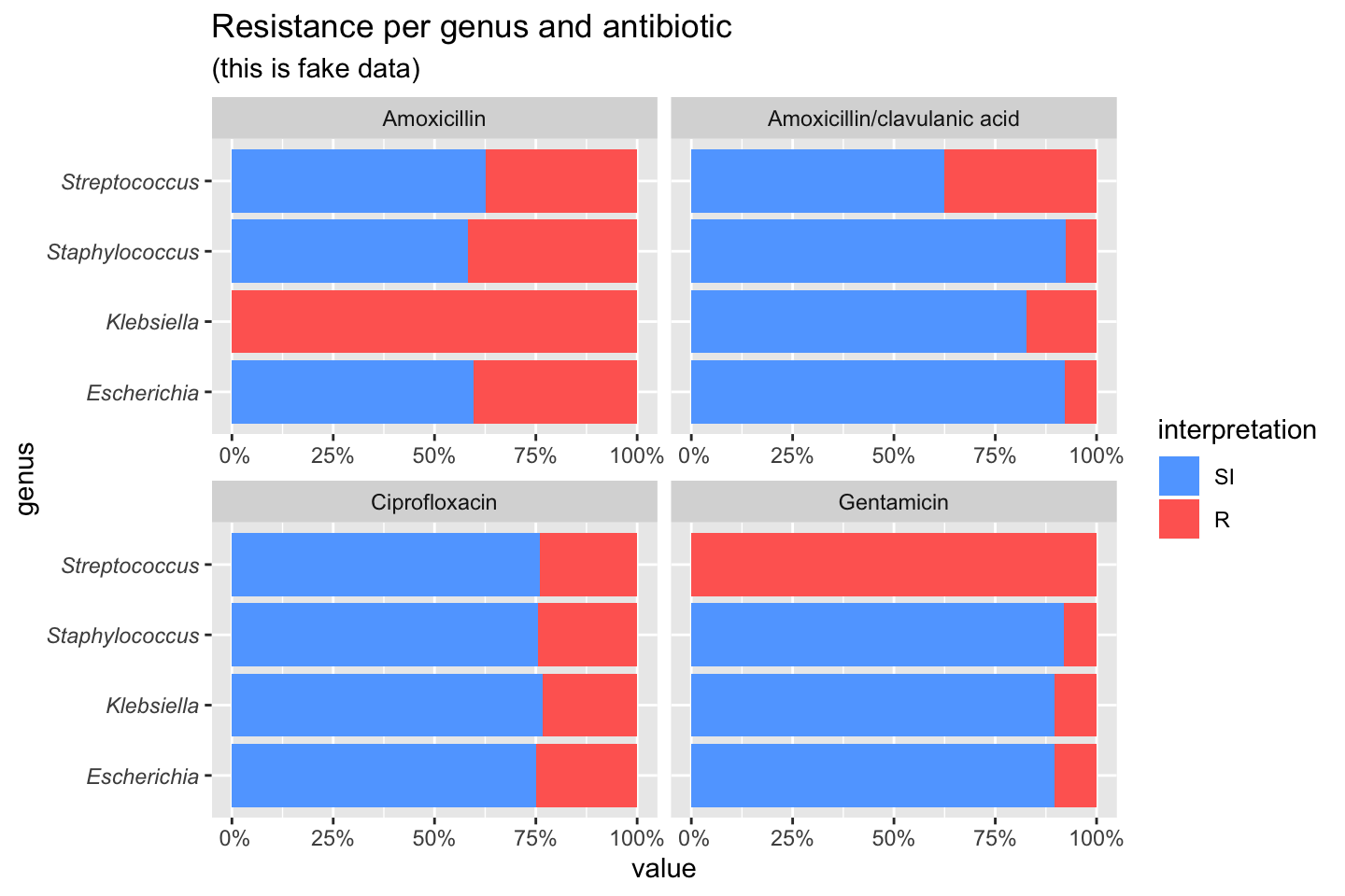
To simplify this, we also created the ggplot_rsi() function, which combines almost all above functions:
data_1st %>%
  group_by(genus) %>%
  ggplot_rsi(x = "genus",
             facet = "antibiotic",
             breaks = 0:4 * 25,
             datalabels = FALSE) +
  coord_flip()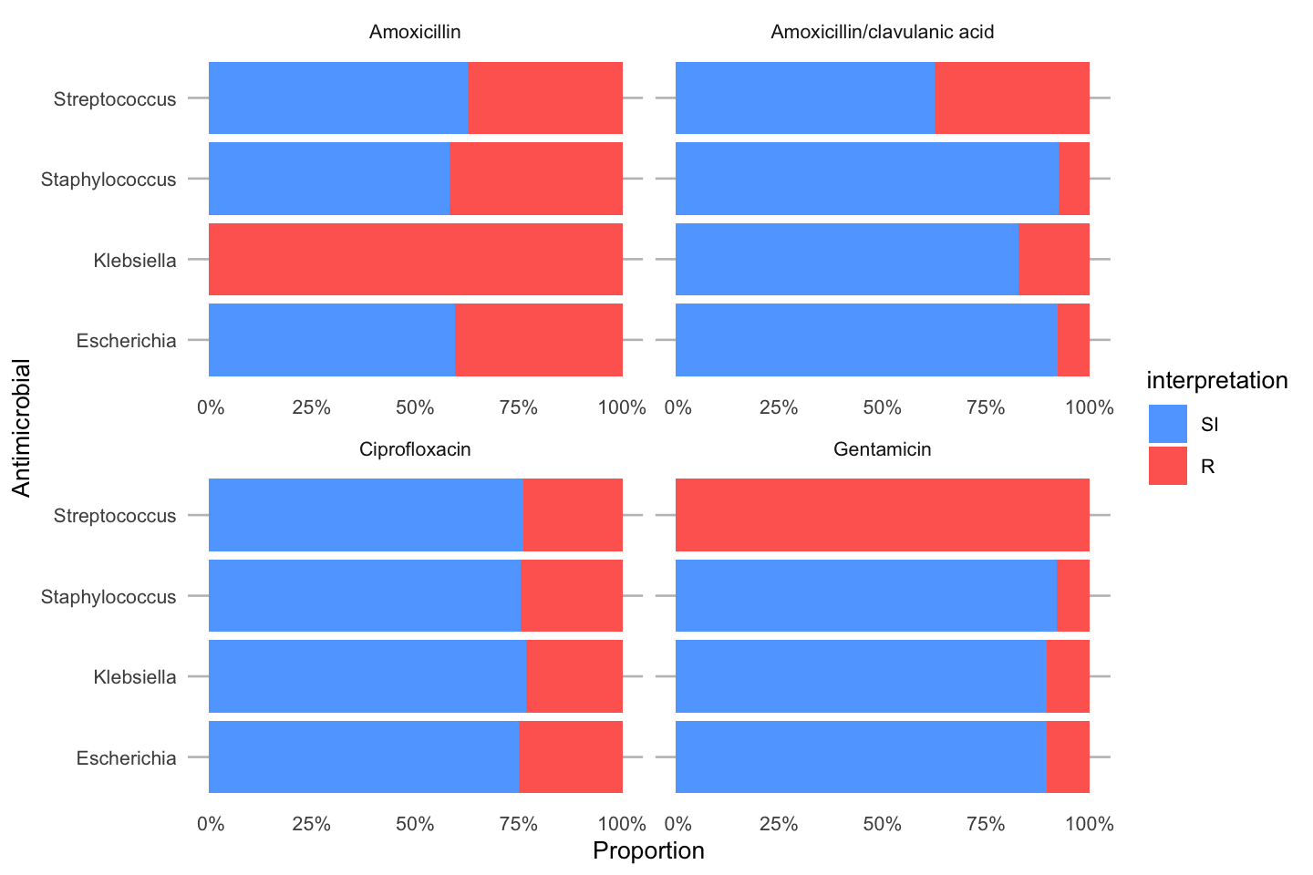
Independence test
The next example uses the included example_isolates, which is an anonymised data set containing 2,000 microbial blood culture isolates with their full antibiograms found in septic patients in 4 different hospitals in the Netherlands, between 2001 and 2017. This data.frame can be used to practice AMR analysis.
We will compare the resistance to fosfomycin (column FOS) in hospital A and D. The input for the fisher.test() can be retrieved with a transformation like this:
check_FOS <- example_isolates %>%
  filter(hospital_id %in% c("A", "D")) %>% # filter on only hospitals A and D
  select(hospital_id, FOS) %>%             # select the hospitals and fosfomycin
  group_by(hospital_id) %>%                # group on the hospitals
  count_df(combine_SI = TRUE) %>%          # count all isolates per group (hospital_id)
  tidyr::spread(hospital_id, value) %>%    # transform output so A and D are columns
  select(A, D) %>%                         # and select these only
  as.matrix()                              # transform to good old matrix for fisher.test()

check_FOS
#       A  D
# [1,] 25 77
# [2,] 24 33
We can apply the test now with:
# do Fisher's Exact Test
fisher.test(check_FOS)
#
#   Fisher's Exact Test for Count Data
#
# data:  check_FOS
# p-value = 0.03104
# alternative hypothesis: true odds ratio is not equal to 1
# 95 percent confidence interval:
#  0.2111489 0.9485124
# sample estimates:
# odds ratio
#  0.4488318
As can be seen, the p value is 0.031, which means that the fosfomycin resistances found in hospital A and D are really different.