How to predict antimicrobial resistance
Source:vignettes/resistance_predict.Rmd
resistance_predict.RmdNeeded R packages
As with many uses in R, we need some additional packages for AMR data analysis. Our package works closely together with the tidyverse packages dplyr and ggplot2 by Dr Hadley Wickham. The tidyverse tremendously improves the way we conduct data science - it allows for a very natural way of writing syntaxes and creating beautiful plots in R.
Our AMR package depends on these packages and even extends their use and functions.
Prediction analysis
Our package contains a function resistance_predict(), which takes the same input as functions for other AMR data analysis. Based on a date column, it calculates cases per year and uses a regression model to predict antimicrobial resistance.
It is basically as easy as:
# resistance prediction of piperacillin/tazobactam (TZP):
resistance_predict(tbl = example_isolates, col_date = "date", col_ab = "TZP", model = "binomial")

# or:
example_isolates %>%
  resistance_predict(col_ab = "TZP",
                     model  "binomial")

# to bind it to object 'predict_TZP' for example:
predict_TZP <- example_isolates %>%
  resistance_predict(col_ab = "TZP",
                     model = "binomial")
The function will look for a date column itself if col_date is not set.
When running any of these commands, a summary of the regression model will be printed unless using resistance_predict(..., info = FALSE).
# ℹ Using column 'date' as input for `col_date`.This text is only a printed summary - the actual result (output) of the function is a data.frame containing for each year: the number of observations, the actual observed resistance, the estimated resistance and the standard error below and above the estimation:
predict_TZP
#    year      value    se_min    se_max observations   observed  estimated
# 1  2002 0.20000000        NA        NA           15 0.20000000 0.05616378
# 2  2003 0.06250000        NA        NA           32 0.06250000 0.06163839
# 3  2004 0.08536585        NA        NA           82 0.08536585 0.06760841
# 4  2005 0.05000000        NA        NA           60 0.05000000 0.07411100
# 5  2006 0.05084746        NA        NA           59 0.05084746 0.08118454
# 6  2007 0.12121212        NA        NA           66 0.12121212 0.08886843
# 7  2008 0.04166667        NA        NA           72 0.04166667 0.09720264
# 8  2009 0.01639344        NA        NA           61 0.01639344 0.10622731
# 9  2010 0.05660377        NA        NA           53 0.05660377 0.11598223
# 10 2011 0.18279570        NA        NA           93 0.18279570 0.12650615
# 11 2012 0.30769231        NA        NA           65 0.30769231 0.13783610
# 12 2013 0.06896552        NA        NA           58 0.06896552 0.15000651
# 13 2014 0.10000000        NA        NA           60 0.10000000 0.16304829
# 14 2015 0.23636364        NA        NA           55 0.23636364 0.17698785
# 15 2016 0.22619048        NA        NA           84 0.22619048 0.19184597
# 16 2017 0.16279070        NA        NA           86 0.16279070 0.20763675
# 17 2018 0.22436641 0.1938710 0.2548618           NA         NA 0.22436641
# 18 2019 0.24203228 0.2062911 0.2777735           NA         NA 0.24203228
# 19 2020 0.26062172 0.2191758 0.3020676           NA         NA 0.26062172
# 20 2021 0.28011130 0.2325557 0.3276669           NA         NA 0.28011130
# 21 2022 0.30046606 0.2464567 0.3544755           NA         NA 0.30046606
# 22 2023 0.32163907 0.2609011 0.3823771           NA         NA 0.32163907
# 23 2024 0.34357130 0.2759081 0.4112345           NA         NA 0.34357130
# 24 2025 0.36619175 0.2914934 0.4408901           NA         NA 0.36619175
# 25 2026 0.38941799 0.3076686 0.4711674           NA         NA 0.38941799
# 26 2027 0.41315710 0.3244399 0.5018743           NA         NA 0.41315710
# 27 2028 0.43730688 0.3418075 0.5328063           NA         NA 0.43730688
# 28 2029 0.46175755 0.3597639 0.5637512           NA         NA 0.46175755
# 29 2030 0.48639359 0.3782932 0.5944939           NA         NA 0.48639359
# 30 2031 0.51109592 0.3973697 0.6248221           NA         NA 0.51109592
The function plot is available in base R, and can be extended by other packages to depend the output based on the type of input. We extended its function to cope with resistance predictions:
plot(predict_TZP)
This is the fastest way to plot the result. It automatically adds the right axes, error bars, titles, number of available observations and type of model.
We also support the ggplot2 package with our custom function ggplot_rsi_predict() to create more appealing plots:
ggplot_rsi_predict(predict_TZP)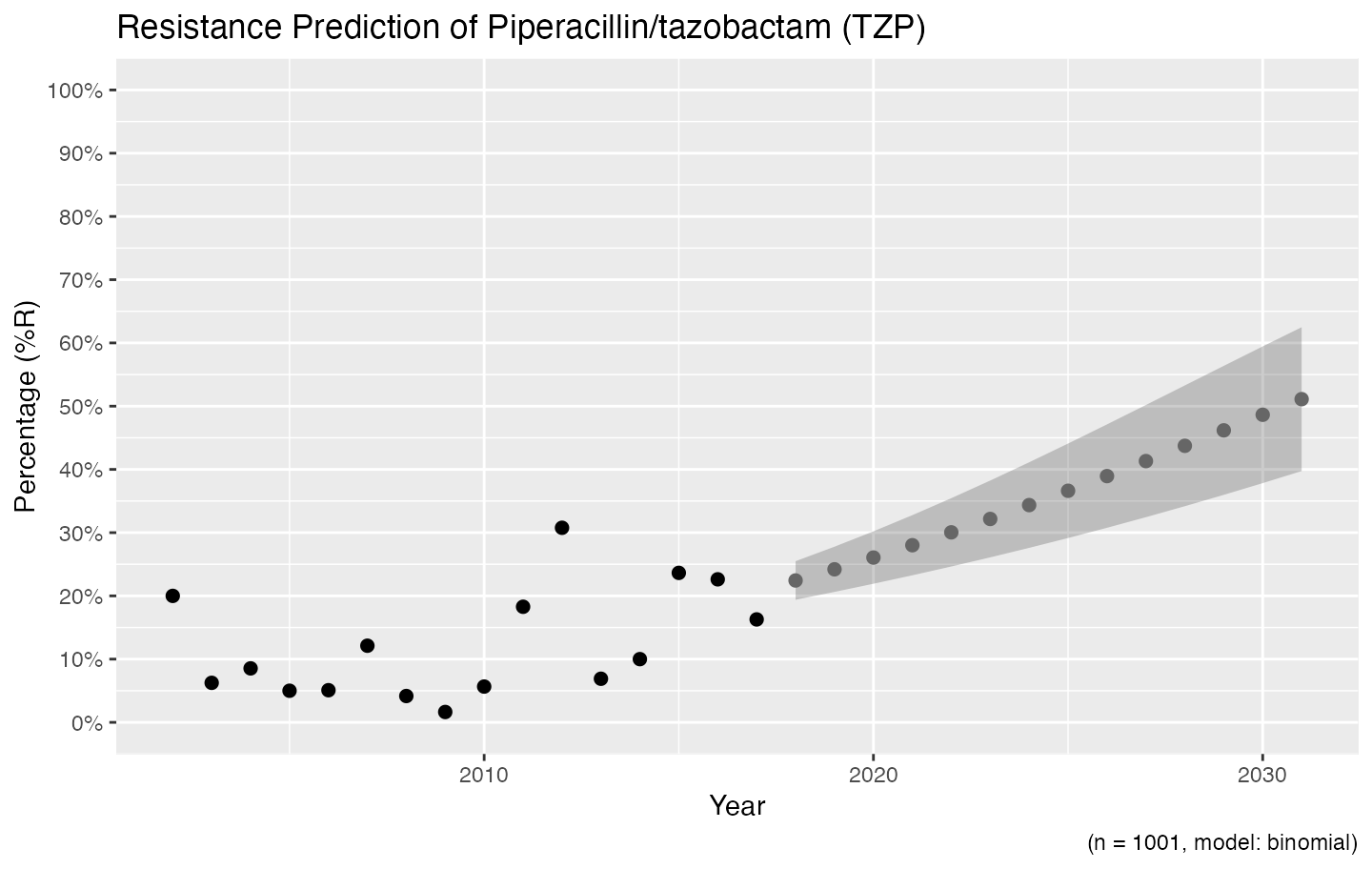
# choose for error bars instead of a ribbon
ggplot_rsi_predict(predict_TZP, ribbon = FALSE)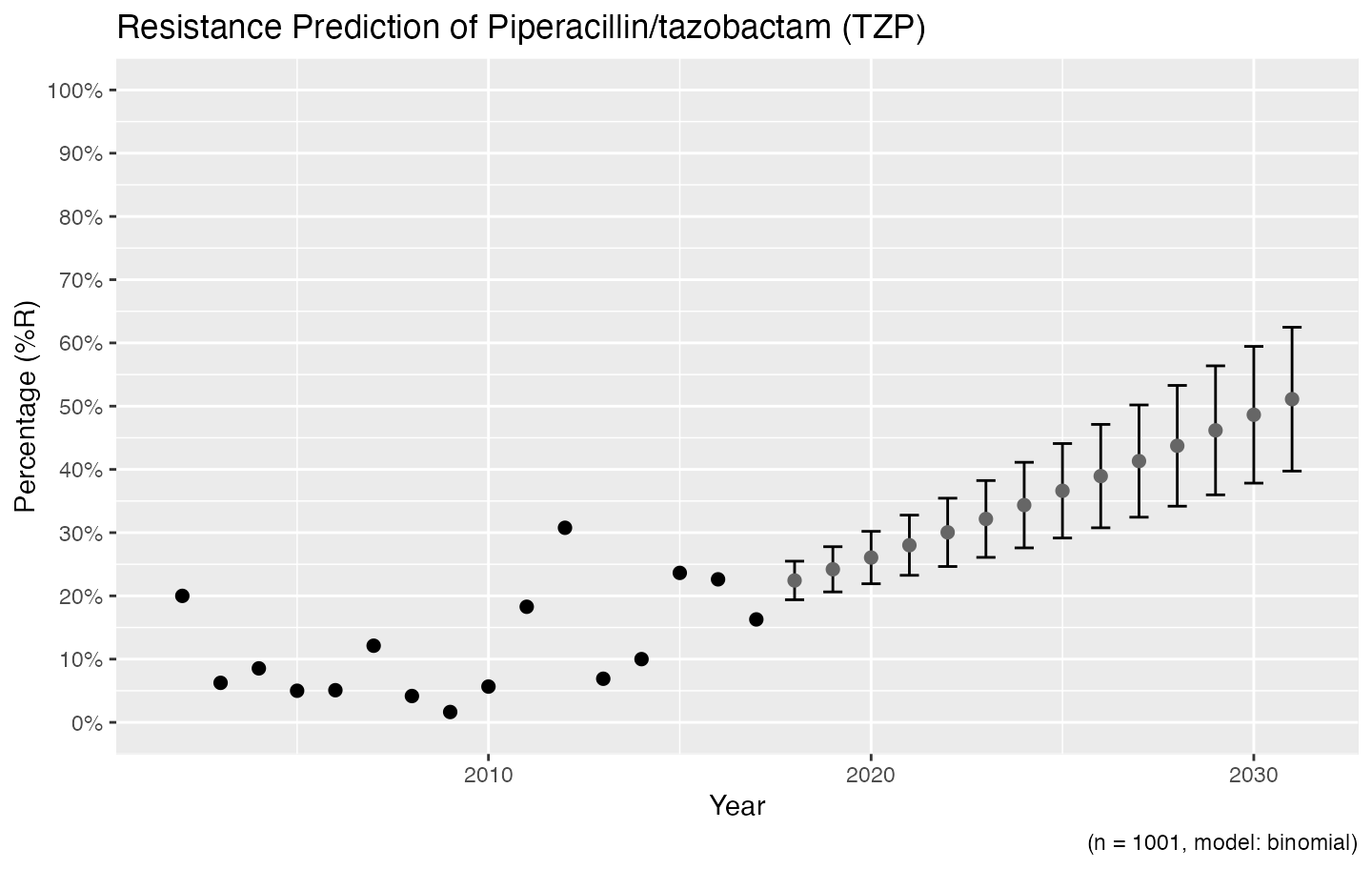
Choosing the right model
Resistance is not easily predicted; if we look at vancomycin resistance in Gram-positive bacteria, the spread (i.e. standard error) is enormous:
example_isolates %>%
  filter(mo_gramstain(mo, language = NULL) == "Gram-positive") %>%
  resistance_predict(col_ab = "VAN", year_min = 2010, info = FALSE, model = "binomial") %>%
  ggplot_rsi_predict()
# ℹ Using column 'date' as input for `col_date`.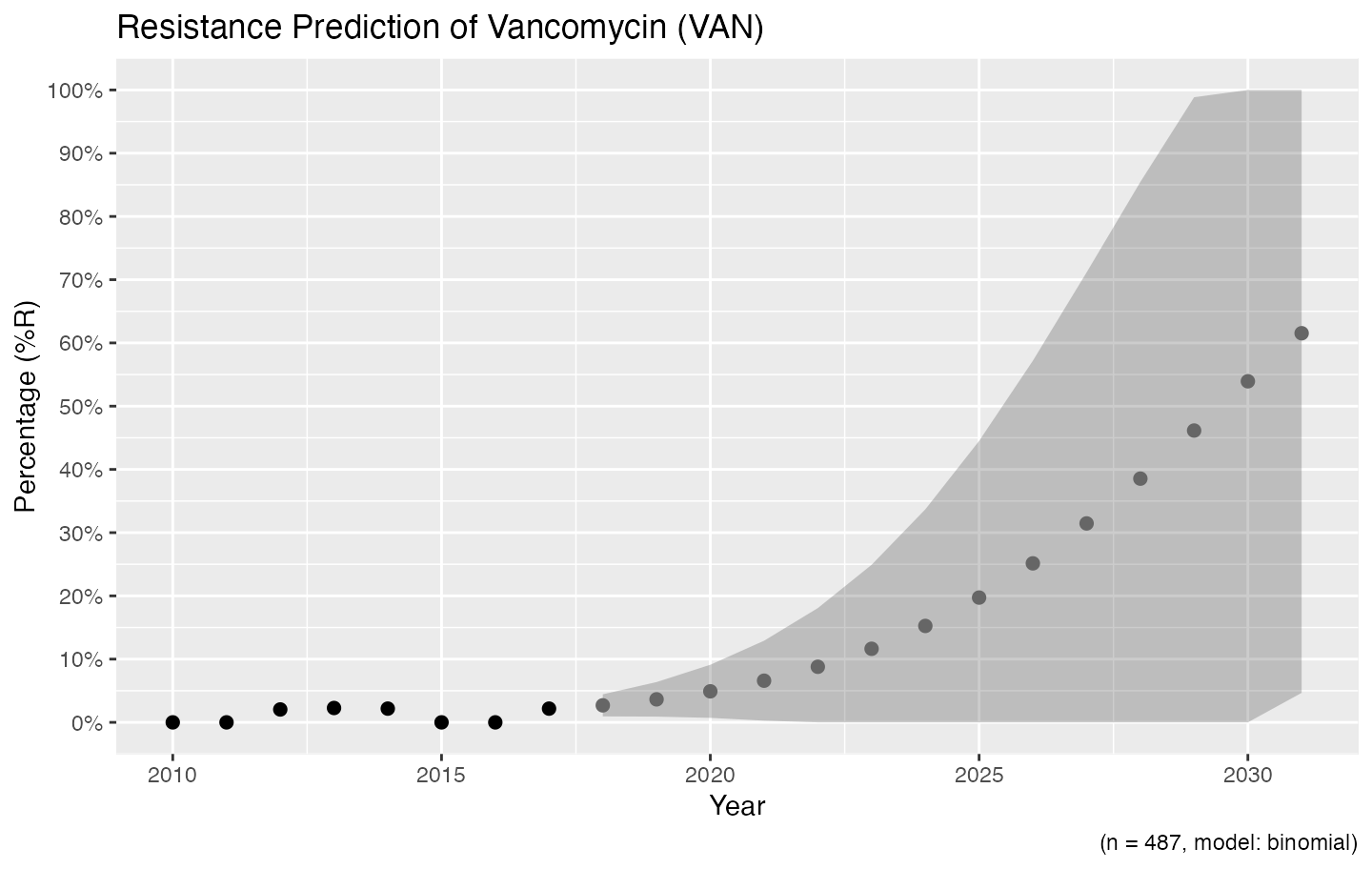
Vancomycin resistance could be 100% in ten years, but might also stay around 0%.
You can define the model with the model parameter. The model chosen above is a generalised linear regression model using a binomial distribution, assuming that a period of zero resistance was followed by a period of increasing resistance leading slowly to more and more resistance.
Valid values are:
| Input values | Function used by R | Type of model |
|---|---|---|
"binomial" or "binom" or "logit"
|
glm(..., family = binomial) |
Generalised linear model with binomial distribution |
"loglin" or "poisson"
|
glm(..., family = poisson) |
Generalised linear model with poisson distribution |
"lin" or "linear"
|
lm() |
Linear model |
For the vancomycin resistance in Gram-positive bacteria, a linear model might be more appropriate since no binomial distribution is to be expected based on the observed years:
example_isolates %>%
  filter(mo_gramstain(mo, language = NULL) == "Gram-positive") %>%
  resistance_predict(col_ab = "VAN", year_min = 2010, info = FALSE, model = "linear") %>%
  ggplot_rsi_predict()
# ℹ Using column 'date' as input for `col_date`.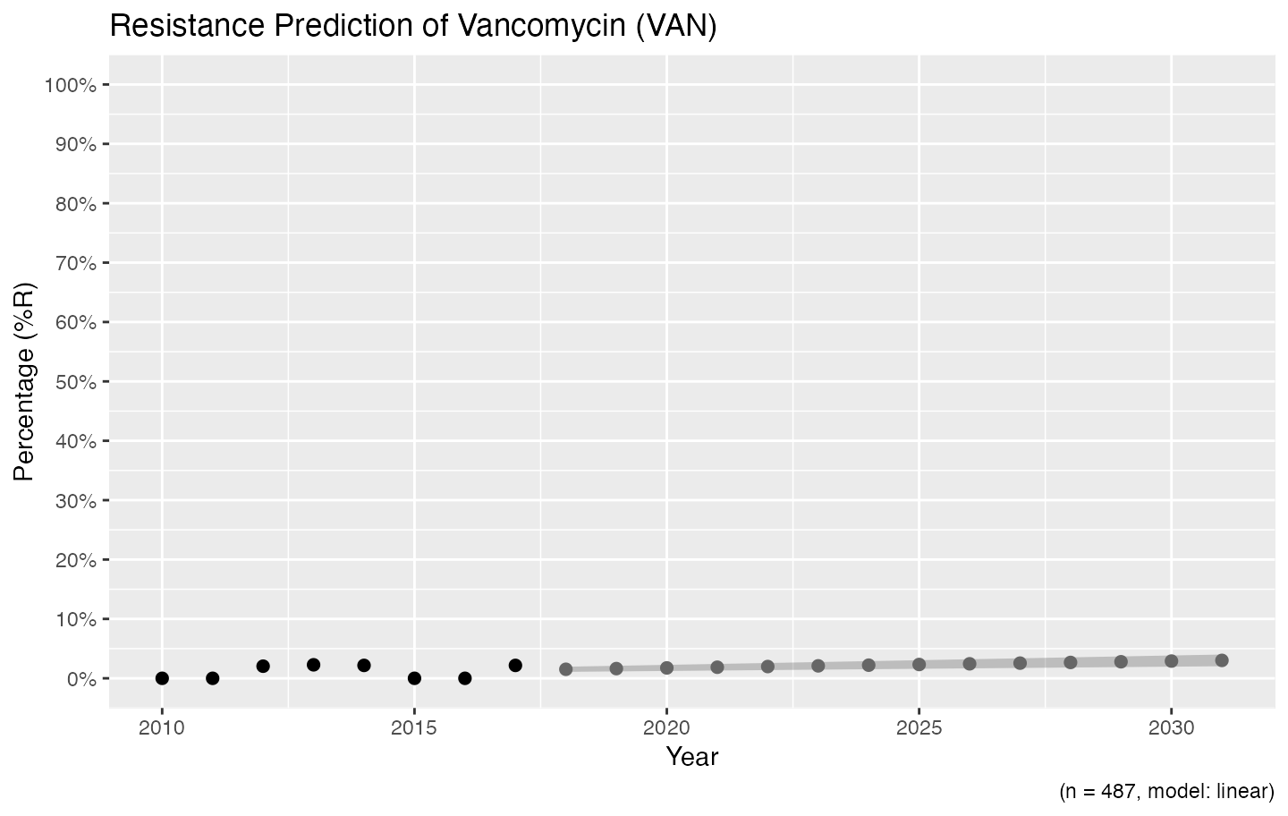
This seems more likely, doesn’t it?
The model itself is also available from the object, as an attribute:
model <- attributes(predict_TZP)$model

summary(model)$family
#
# Family: binomial
# Link function: logit

summary(model)$coefficients
#                  Estimate  Std. Error   z value     Pr(>|z|)
# (Intercept) -200.67944891 46.17315349 -4.346237 1.384932e-05
# year           0.09883005  0.02295317  4.305725 1.664395e-05