Benchmarks
Matthijs S. Berends
20 December 2019
benchmarks.RmdOne of the most important features of this package is the complete microbial taxonomic database, supplied by the Catalogue of Life. We created a function as.mo() that transforms any user input value to a valid microbial ID by using intelligent rules combined with the taxonomic tree of Catalogue of Life.
Using the microbenchmark package, we can review the calculation performance of this function. Its function microbenchmark() runs different input expressions independently of each other and measures their time-to-result.
FALSE
In the next test, we try to ‘coerce’ different input values into the microbial code of Staphylococcus aureus. Coercion is a computational process of forcing output based on an input. For microorganism names, coercing user input to taxonomically valid microorganism names is crucial to ensure correct interpretation and to enable grouping based on taxonomic properties.
The actual result is the same every time: it returns its microorganism code B_STPHY_AURS (B stands for Bacteria, the taxonomic kingdom).
But the calculation time differs a lot:
S.aureus <- microbenchmark(
  as.mo("sau"), # WHONET code
  as.mo("stau"),
  as.mo("STAU"),
  as.mo("staaur"),
  as.mo("STAAUR"),
  as.mo("S. aureus"),
  as.mo("S aureus"),
  as.mo("Staphylococcus aureus"), # official taxonomic name
  as.mo("Staphylococcus aureus (MRSA)"), # additional text
  as.mo("Sthafilokkockus aaureuz"), # incorrect spelling
  as.mo("MRSA"), # Methicillin Resistant S. aureus
  as.mo("VISA"), # Vancomycin Intermediate S. aureus
  as.mo("VRSA"), # Vancomycin Resistant S. aureus
  as.mo(22242419), # Catalogue of Life ID
  times = 10)
print(S.aureus, unit = "ms", signif = 2)
# Unit: milliseconds
#                                   expr   min    lq  mean median    uq max neval
#                           as.mo("sau")   9.2   9.4   9.7    9.6  10.0  11    10
#                          as.mo("stau")  32.0  34.0  43.0   37.0  58.0  66    10
#                          as.mo("STAU")  34.0  34.0  40.0   35.0  36.0  65    10
#                        as.mo("staaur")   9.2   9.3  12.0    9.8  11.0  33    10
#                        as.mo("STAAUR")   9.1   9.5  12.0    9.6   9.9  35    10
#                     as.mo("S. aureus")  24.0  25.0  34.0   28.0  48.0  55    10
#                      as.mo("S aureus")  24.0  24.0  32.0   26.0  32.0  55    10
#         as.mo("Staphylococcus aureus")   4.6   4.7   9.7    4.8   5.5  30    10
#  as.mo("Staphylococcus aureus (MRSA)") 620.0 630.0 670.0  650.0 680.0 840    10
#       as.mo("Sthafilokkockus aaureuz") 320.0 330.0 370.0  350.0 410.0 470    10
#                          as.mo("MRSA")   9.2   9.8  17.0   10.0  32.0  37    10
#                          as.mo("VISA")  19.0  19.0  23.0   20.0  23.0  49    10
#                          as.mo("VRSA")  19.0  20.0  26.0   22.0  25.0  46    10
#                        as.mo(22242419)  18.0  19.0  23.0   20.0  24.0  43    10
In the table above, all measurements are shown in milliseconds (thousands of seconds). A value of 5 milliseconds means it can determine 200 input values per second. It case of 100 milliseconds, this is only 10 input values per second. The second input is the only one that has to be looked up thoroughly. All the others are known codes (the first one is a WHONET code) or common laboratory codes, or common full organism names like the last one. Full organism names are always preferred.
To achieve this speed, the as.mo function also takes into account the prevalence of human pathogenic microorganisms. The downside is of course that less prevalent microorganisms will be determined less fast. See this example for the ID of Methanosarcina semesiae (B_MTHNSR_SEMS), a bug probably never found before in humans:
M.semesiae <- microbenchmark(as.mo("metsem"),
                             as.mo("METSEM"),
                             as.mo("M. semesiae"),
                             as.mo("M.  semesiae"),
                             as.mo("Methanosarcina semesiae"),
                             times = 10)
print(M.semesiae, unit = "ms", signif = 4)
# Unit: milliseconds
#                              expr      min       lq    mean   median      uq
#                   as.mo("metsem") 1424.000 1452.000 1483.00 1489.000 1518.00
#                   as.mo("METSEM") 1342.000 1434.000 1477.00 1491.000 1522.00
#              as.mo("M. semesiae") 2104.000 2163.000 2180.00 2196.000 2202.00
#             as.mo("M.  semesiae") 2111.000 2148.000 2168.00 2170.000 2183.00
#  as.mo("Methanosarcina semesiae")    5.309    5.483   13.19    5.854   28.63
#      max neval
#  1554.00    10
#  1584.00    10
#  2214.00    10
#  2208.00    10
#    32.07    10
That takes 15.5 times as much time on average. A value of 100 milliseconds means it can only determine ~10 different input values per second. We can conclude that looking up arbitrary codes of less prevalent microorganisms is the worst way to go, in terms of calculation performance. Full names (like Methanosarcina semesiae) are always very fast and only take some thousands of seconds to coerce - they are the most probable input from most data sets.
In the figure below, we compare Escherichia coli (which is very common) with Prevotella brevis (which is moderately common) and with Methanosarcina semesiae (which is uncommon):
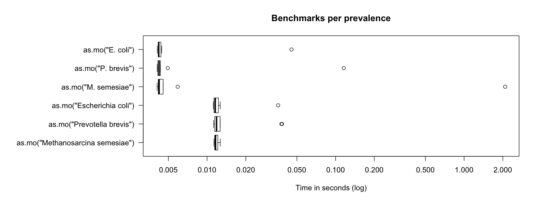
In reality, the as.mo() functions learns from its own output to speed up determinations for next times. In below figure, this effect was disabled to show the difference with the boxplot above:
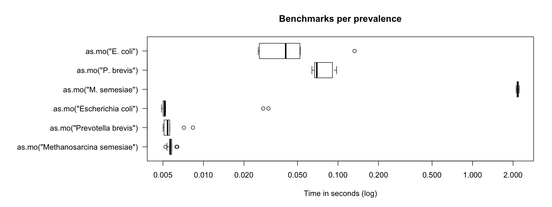
The highest outliers are the first times. All next determinations were done in only thousands of seconds.
Uncommon microorganisms take a lot more time than common microorganisms. To relieve this pitfall and further improve performance, two important calculations take almost no time at all: repetitive results and already precalculated results.
Repetitive results
Repetitive results are unique values that are present more than once. Unique values will only be calculated once by as.mo(). We will use mo_name() for this test - a helper function that returns the full microbial name (genus, species and possibly subspecies) which uses as.mo() internally.
library(dplyr)
# take all MO codes from the example_isolates data set
x <- example_isolates$mo %>%
  # keep only the unique ones
  unique() %>%
  # pick 50 of them at random
  sample(50) %>%
  # paste that 10,000 times
  rep(10000) %>%
  # scramble it
  sample()

# got indeed 50 times 10,000 = half a million?
length(x)
# [1] 500000

# and how many unique values do we have?
n_distinct(x)
# [1] 50

# now let's see:
run_it <- microbenchmark(mo_name(x),
                         times = 10)
print(run_it, unit = "ms", signif = 3)
# Unit: milliseconds
#        expr min  lq mean median  uq max neval
#  mo_name(x) 620 645  659    660 672 700    10
So transforming 500,000 values (!!) of 50 unique values only takes 0.66 seconds (660 ms). You only lose time on your unique input values.
Precalculated results
What about precalculated results? If the input is an already precalculated result of a helper function like mo_name(), it almost doesn’t take any time at all (see ‘C’ below):
run_it <- microbenchmark(A = mo_name("B_STPHY_AURS"),
                         B = mo_name("S. aureus"),
                         C = mo_name("Staphylococcus aureus"),
                         times = 10)
print(run_it, unit = "ms", signif = 3)
# Unit: milliseconds
#  expr    min     lq   mean median     uq    max neval
#     A  6.360  6.400  6.770  6.500  6.720  8.590    10
#     B 24.800 25.100 32.500 28.400 30.400 54.200    10
#     C  0.704  0.747  0.777  0.785  0.814  0.817    10
So going from mo_name("Staphylococcus aureus") to "Staphylococcus aureus" takes 0.0008 seconds - it doesn’t even start calculating if the result would be the same as the expected resulting value. That goes for all helper functions:
run_it <- microbenchmark(A = mo_species("aureus"),
                         B = mo_genus("Staphylococcus"),
                         C = mo_name("Staphylococcus aureus"),
                         D = mo_family("Staphylococcaceae"),
                         E = mo_order("Bacillales"),
                         F = mo_class("Bacilli"),
                         G = mo_phylum("Firmicutes"),
                         H = mo_kingdom("Bacteria"),
                         times = 10)
print(run_it, unit = "ms", signif = 3)
# Unit: milliseconds
#  expr   min    lq  mean median    uq   max neval
#     A 0.450 0.453 0.471  0.467 0.491 0.497    10
#     B 0.492 0.500 0.508  0.507 0.508 0.549    10
#     C 0.725 0.770 0.793  0.799 0.819 0.849    10
#     D 0.492 0.494 0.505  0.501 0.510 0.549    10
#     E 0.450 0.460 0.466  0.462 0.466 0.507    10
#     F 0.441 0.450 0.459  0.458 0.467 0.491    10
#     G 0.444 0.450 0.463  0.464 0.470 0.492    10
#     H 0.448 0.458 0.481  0.459 0.463 0.658    10
Of course, when running mo_phylum("Firmicutes") the function has zero knowledge about the actual microorganism, namely S. aureus. But since the result would be "Firmicutes" too, there is no point in calculating the result. And because this package ‘knows’ all phyla of all known bacteria (according to the Catalogue of Life), it can just return the initial value immediately.
Results in other languages
When the system language is non-English and supported by this AMR package, some functions will have a translated result. This almost does’t take extra time:
mo_name("CoNS", language = "en") # or just mo_name("CoNS") on an English system
# [1] "Coagulase-negative Staphylococcus (CoNS)"

mo_name("CoNS", language = "es") # or just mo_name("CoNS") on a Spanish system
# [1] "Staphylococcus coagulasa negativo (SCN)"

mo_name("CoNS", language = "nl") # or just mo_name("CoNS") on a Dutch system
# [1] "Coagulase-negatieve Staphylococcus (CNS)"

run_it <- microbenchmark(en = mo_name("CoNS", language = "en"),
                         de = mo_name("CoNS", language = "de"),
                         nl = mo_name("CoNS", language = "nl"),
                         es = mo_name("CoNS", language = "es"),
                         it = mo_name("CoNS", language = "it"),
                         fr = mo_name("CoNS", language = "fr"),
                         pt = mo_name("CoNS", language = "pt"),
                         times = 10)
print(run_it, unit = "ms", signif = 4)
# Unit: milliseconds
#  expr   min    lq  mean median    uq   max neval
#    en 20.20 20.36 25.81  20.55 26.48 44.15    10
#    de 21.79 21.97 29.74  22.27 45.35 49.38    10
#    nl 27.24 27.39 28.69  27.85 28.68 35.16    10
#    es 21.48 21.51 27.65  21.97 22.85 55.52    10
#    it 21.92 21.95 24.77  22.11 22.63 47.75    10
#    fr 21.46 21.55 25.53  22.59 23.05 50.67    10
#    pt 21.44 21.79 24.62  21.88 23.07 46.35    10
Currently supported are German, Dutch, Spanish, Italian, French and Portuguese.