This page was entirely written by our AMR for R Assistant, a ChatGPT manually-trained model able to answer any question about the AMR package.
Antimicrobial resistance (AMR) is a global health crisis, and
understanding resistance patterns is crucial for managing effective
treatments. The AMR R package provides robust tools for
analysing AMR data, including convenient antibiotic selector functions
like aminoglycosides() and betalactams(). In
this post, we will explore how to use the tidymodels
framework to predict resistance patterns in the
example_isolates dataset.
By leveraging the power of tidymodels and the
AMR package, we’ll build a reproducible machine learning
workflow to predict the Gramstain of the microorganism to two important
antibiotic classes: aminoglycosides and beta-lactams.
Objective
Our goal is to build a predictive model using the
tidymodels framework to determine the Gramstain of the
microorganism based on microbial data. We will:
- Preprocess data using the selector functions
aminoglycosides()andbetalactams(). - Define a logistic regression model for prediction.
- Use a structured
tidymodelsworkflow to preprocess, train, and evaluate the model.
Data Preparation
We begin by loading the required libraries and preparing the
example_isolates dataset from the AMR
package.
# Load required libraries
library(AMR)          # For AMR data analysis
library(tidymodels)   # For machine learning workflows, and data manipulation (dplyr, tidyr, ...)
#> ── Attaching packages ────────────────────────────────────── tidymodels 1.3.0 ──
#> ✔ broom        1.0.7     ✔ recipes      1.1.1
#> ✔ dials        1.4.0     ✔ rsample      1.2.1
#> ✔ dplyr        1.1.4     ✔ tibble       3.2.1
#> ✔ ggplot2      3.5.1     ✔ tidyr        1.3.1
#> ✔ infer        1.0.7     ✔ tune         1.3.0
#> ✔ modeldata    1.4.0     ✔ workflows    1.2.0
#> ✔ parsnip      1.3.0     ✔ workflowsets 1.1.0
#> ✔ purrr        1.0.4     ✔ yardstick    1.3.2
#> ── Conflicts ───────────────────────────────────────── tidymodels_conflicts() ──
#> ✖ purrr::discard() masks scales::discard()
#> ✖ dplyr::filter()  masks stats::filter()
#> ✖ dplyr::lag()     masks stats::lag()
#> ✖ recipes::step()  masks stats::step()

# Select relevant columns for prediction
data <- example_isolates %>%
  # select AB results dynamically
  select(mo, aminoglycosides(), betalactams()) %>%
  # replace NAs with NI (not-interpretable)
   mutate(across(where(is.sir),
                 ~replace_na(.x, "NI")),
          # make factors of SIR columns
          across(where(is.sir),
                 as.integer),
          # get Gramstain of microorganisms
          mo = as.factor(mo_gramstain(mo))) %>%
  # drop NAs - the ones without a Gramstain (fungi, etc.)
  drop_na()
#> ℹ For aminoglycosides() using columns 'GEN' (gentamicin), 'TOB'
#>   (tobramycin), 'AMK' (amikacin), and 'KAN' (kanamycin)
#> ℹ For betalactams() using columns 'PEN' (benzylpenicillin), 'OXA'
#>   (oxacillin), 'FLC' (flucloxacillin), 'AMX' (amoxicillin), 'AMC'
#>   (amoxicillin/clavulanic acid), 'AMP' (ampicillin), 'TZP'
#>   (piperacillin/tazobactam), 'CZO' (cefazolin), 'FEP' (cefepime), 'CXM'
#>   (cefuroxime), 'FOX' (cefoxitin), 'CTX' (cefotaxime), 'CAZ' (ceftazidime),
#>   'CRO' (ceftriaxone), 'IPM' (imipenem), and 'MEM' (meropenem)
Explanation:
-
aminoglycosides()andbetalactams()dynamically select columns for antimicrobials in these classes. -
drop_na()ensures the model receives complete cases for training.
Defining the Workflow
We now define the tidymodels workflow, which consists of
three steps: preprocessing, model specification, and fitting.
1. Preprocessing with a Recipe
We create a recipe to preprocess the data for modelling.
# Define the recipe for data preprocessing
resistance_recipe <- recipe(mo ~ ., data = data) %>%
  step_corr(c(aminoglycosides(), betalactams()), threshold = 0.9)
resistance_recipe
#>
#> ── Recipe ──────────────────────────────────────────────────────────────────────
#>
#> ── Inputs
#> Number of variables by role
#> outcome:    1
#> predictor: 20
#>
#> ── Operations
#> • Correlation filter on: c(aminoglycosides(), betalactams())
For a recipe that includes at least one preprocessing operation, like
we have with step_corr(), the necessary parameters can be
estimated from a training set using prep():
prep(resistance_recipe)
#> ℹ For aminoglycosides() using columns 'GEN' (gentamicin), 'TOB'
#>   (tobramycin), 'AMK' (amikacin), and 'KAN' (kanamycin)
#> ℹ For betalactams() using columns 'PEN' (benzylpenicillin), 'OXA'
#>   (oxacillin), 'FLC' (flucloxacillin), 'AMX' (amoxicillin), 'AMC'
#>   (amoxicillin/clavulanic acid), 'AMP' (ampicillin), 'TZP'
#>   (piperacillin/tazobactam), 'CZO' (cefazolin), 'FEP' (cefepime), 'CXM'
#>   (cefuroxime), 'FOX' (cefoxitin), 'CTX' (cefotaxime), 'CAZ' (ceftazidime),
#>   'CRO' (ceftriaxone), 'IPM' (imipenem), and 'MEM' (meropenem)
#>
#> ── Recipe ──────────────────────────────────────────────────────────────────────
#>
#> ── Inputs
#> Number of variables by role
#> outcome:    1
#> predictor: 20
#>
#> ── Training information
#> Training data contained 1968 data points and no incomplete rows.
#>
#> ── Operations
#> • Correlation filter on: AMX CTX | Trained
Explanation:
-
recipe(mo ~ ., data = data)will take themocolumn as outcome and all other columns as predictors. -
step_corr()removes predictors (i.e., antibiotic columns) that have a higher correlation than 90%.
Notice how the recipe contains just the antibiotic selector functions
- no need to define the columns specifically. In the preparation
(retrieved with prep()) we can see that the columns or
variables ‘AMX’ and ‘CTX’ were removed as they correlate too much with
existing, other variables.
2. Specifying the Model
We define a logistic regression model since resistance prediction is a binary classification task.
# Specify a logistic regression model
logistic_model <- logistic_reg() %>%
  set_engine("glm") # Use the Generalized Linear Model engine
logistic_model
#> Logistic Regression Model Specification (classification)
#>
#> Computational engine: glm
Explanation:
-
logistic_reg()sets up a logistic regression model. -
set_engine("glm")specifies the use of R’s built-in GLM engine.
3. Building the Workflow
We bundle the recipe and model together into a workflow,
which organizes the entire modeling process.
# Combine the recipe and model into a workflow
resistance_workflow <- workflow() %>%
  add_recipe(resistance_recipe) %>% # Add the preprocessing recipe
  add_model(logistic_model) # Add the logistic regression model
resistance_workflow
#> ══ Workflow ════════════════════════════════════════════════════════════════════
#> Preprocessor: Recipe
#> Model: logistic_reg()
#>
#> ── Preprocessor ────────────────────────────────────────────────────────────────
#> 1 Recipe Step
#>
#> • step_corr()
#>
#> ── Model ───────────────────────────────────────────────────────────────────────
#> Logistic Regression Model Specification (classification)
#>
#> Computational engine: glm
Training and Evaluating the Model
To train the model, we split the data into training and testing sets. Then, we fit the workflow on the training set and evaluate its performance.
# Split data into training and testing sets
set.seed(123) # For reproducibility
data_split <- initial_split(data, prop = 0.8) # 80% training, 20% testing
training_data <- training(data_split) # Training set
testing_data <- testing(data_split)   # Testing set

# Fit the workflow to the training data
fitted_workflow <- resistance_workflow %>%
  fit(training_data) # Train the model
Explanation:
-
initial_split()splits the data into training and testing sets. -
fit()trains the workflow on the training set.
Notice how in fit(), the antibiotic selector functions
are internally called again. For training, these functions are called
since they are stored in the recipe.
Next, we evaluate the model on the testing data.
# Make predictions on the testing set
predictions <- fitted_workflow %>%
  predict(testing_data)                # Generate predictions
probabilities <- fitted_workflow %>%
  predict(testing_data, type = "prob") # Generate probabilities

predictions <- predictions %>%
  bind_cols(probabilities) %>%
  bind_cols(testing_data) # Combine with true labels

predictions
#> # A tibble: 394 × 24
#>    .pred_class   `.pred_Gram-negative` `.pred_Gram-positive` mo        GEN   TOB
#>    <fct>                         <dbl>                 <dbl> <fct>   <int> <int>
#>  1 Gram-positive              1.07e- 1              8.93e- 1 Gram-p…     5     5
#>  2 Gram-positive              3.17e- 8              1.00e+ 0 Gram-p…     5     1
#>  3 Gram-negative              9.99e- 1              1.42e- 3 Gram-n…     5     5
#>  4 Gram-positive              2.22e-16              1   e+ 0 Gram-p…     5     5
#>  5 Gram-negative              9.46e- 1              5.42e- 2 Gram-n…     5     5
#>  6 Gram-positive              1.07e- 1              8.93e- 1 Gram-p…     5     5
#>  7 Gram-positive              2.22e-16              1   e+ 0 Gram-p…     1     5
#>  8 Gram-positive              2.22e-16              1   e+ 0 Gram-p…     4     4
#>  9 Gram-negative              1   e+ 0              2.22e-16 Gram-n…     1     1
#> 10 Gram-positive              6.05e-11              1.00e+ 0 Gram-p…     4     4
#> # ℹ 384 more rows
#> # ℹ 18 more variables: AMK <int>, KAN <int>, PEN <int>, OXA <int>, FLC <int>,
#> #   AMX <int>, AMC <int>, AMP <int>, TZP <int>, CZO <int>, FEP <int>,
#> #   CXM <int>, FOX <int>, CTX <int>, CAZ <int>, CRO <int>, IPM <int>, MEM <int>

# Evaluate model performance
metrics <- predictions %>%
  metrics(truth = mo, estimate = .pred_class) # Calculate performance metrics

metrics
#> # A tibble: 2 × 3
#>   .metric  .estimator .estimate
#>   <chr>    <chr>          <dbl>
#> 1 accuracy binary         0.995
#> 2 kap      binary         0.989
Explanation:
-
predict()generates predictions on the testing set. -
metrics()computes evaluation metrics like accuracy and kappa.
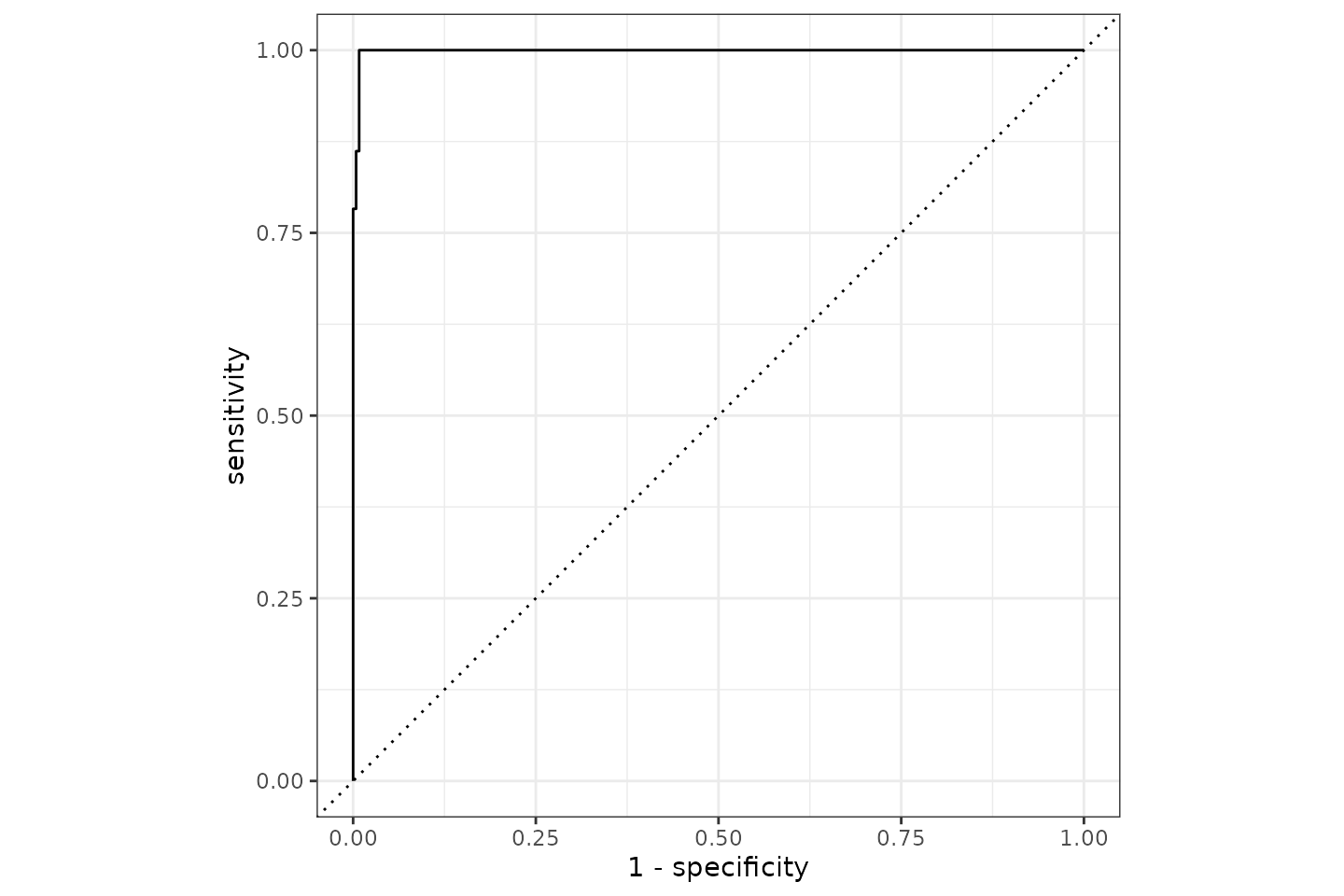
It appears we can predict the Gram based on AMR results with a 99.5% accuracy based on AMR results of aminoglycosides and beta-lactam antibiotics. The ROC curve looks like this:
Conclusion
In this post, we demonstrated how to build a machine learning
pipeline with the tidymodels framework and the
AMR package. By combining selector functions like
aminoglycosides() and betalactams() with
tidymodels, we efficiently prepared data, trained a model,
and evaluated its performance.
This workflow is extensible to other antibiotic classes and resistance patterns, empowering users to analyse AMR data systematically and reproducibly.