Benchmarks
Matthijs S. Berends
21 February 2019
benchmarks.RmdOne of the most important features of this package is the complete microbial taxonomic database, supplied by the Catalogue of Life. We created a function as.mo() that transforms any user input value to a valid microbial ID by using AI (Artificial Intelligence) combined with the taxonomic tree of Catalogue of Life.
Using the microbenchmark package, we can review the calculation performance of this function. Its function microbenchmark() runs different input expressions independently of each other and measures their time-to-result.
In the next test, we try to ‘coerce’ different input values for Staphylococcus aureus. The actual result is the same every time: it returns its MO code B_STPHY_AUR (B stands for Bacteria, the taxonomic kingdom).
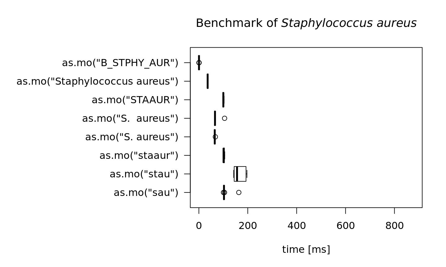
But the calculation time differs a lot. Here, the AI effect can be reviewed best:
S.aureus <- microbenchmark(as.mo("sau"),
                           as.mo("stau"),
                           as.mo("staaur"),
                           as.mo("S. aureus"),
                           as.mo("S.  aureus"),
                           as.mo("STAAUR"),
                           as.mo("Staphylococcus aureus"),
                           as.mo("B_STPHY_AUR"),
                           times = 10)
print(S.aureus, unit = "ms", signif = 2)
#> Unit: milliseconds
#>                            expr    min     lq   mean median     uq    max
#>                    as.mo("sau") 100.00 100.00 110.00 100.00 100.00 160.00
#>                   as.mo("stau") 140.00 140.00 170.00 160.00 190.00 200.00
#>                 as.mo("staaur")  99.00 100.00 100.00 100.00 100.00 110.00
#>              as.mo("S. aureus")  64.00  64.00  65.00  65.00  66.00  67.00
#>             as.mo("S.  aureus")  65.00  65.00  70.00  66.00  66.00 110.00
#>                 as.mo("STAAUR")  97.00  98.00 100.00 100.00 100.00 100.00
#>  as.mo("Staphylococcus aureus")  35.00  35.00  36.00  36.00  37.00  38.00
#>            as.mo("B_STPHY_AUR")   0.34   0.47   0.52   0.48   0.56   0.89
#>  neval
#>     10
#>     10
#>     10
#>     10
#>     10
#>     10
#>     10
#>     10
In the table above, all measurements are shown in milliseconds (thousands of seconds). A value of 10 milliseconds means it can determine 100 input values per second. It case of 50 milliseconds, this is only 20 input values per second. The more an input value resembles a full name, the faster the result will be found. In case of as.mo("B_STPHY_AUR"), the input is already a valid MO code, so it only almost takes no time at all (476 millionths of a second).
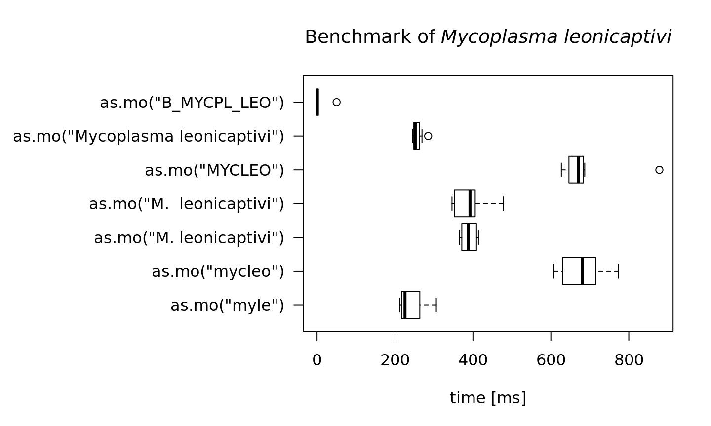
To achieve this speed, the as.mo function also takes into account the prevalence of human pathogenic microorganisms. The downside is of course that less prevalent microorganisms will be determined less fast. See this example for the ID of Mycoplasma leonicaptivi (B_MYCPL_LEO), a bug probably never found before in humans:
M.leonicaptivi <- microbenchmark(as.mo("myle"),
                                 as.mo("mycleo"),
                                 as.mo("M. leonicaptivi"),
                                 as.mo("M.  leonicaptivi"),
                                 as.mo("MYCLEO"),
                                 as.mo("Mycoplasma leonicaptivi"),
                                 as.mo("B_MYCPL_LEO"),
                                 times = 10)
print(M.leonicaptivi, unit = "ms", signif = 2)
#> Unit: milliseconds
#>                              expr    min     lq  mean median     uq max
#>                     as.mo("myle") 210.00 220.00 240.0 230.00 260.00 310
#>                   as.mo("mycleo") 610.00 630.00 680.0 680.00 720.00 770
#>          as.mo("M. leonicaptivi") 370.00 370.00 390.0 390.00 410.00 410
#>         as.mo("M.  leonicaptivi") 350.00 350.00 390.0 390.00 410.00 480
#>                   as.mo("MYCLEO") 630.00 650.00 680.0 670.00 680.00 880
#>  as.mo("Mycoplasma leonicaptivi") 250.00 250.00 260.0 250.00 260.00 290
#>              as.mo("B_MYCPL_LEO")   0.35   0.43   5.6   0.69   0.75  50
#>  neval
#>     10
#>     10
#>     10
#>     10
#>     10
#>     10
#>     10
That takes 4.7 times as much time on average! A value of 100 milliseconds means it can only determine ~10 different input values per second. We can conclude that looking up arbitrary codes of less prevalent microorganisms is the worst way to go, in terms of calculation performance:
par(mar = c(5, 16, 4, 2)) # set more space for left margin text (16)

# highest value on y axis
max_y_axis <- max(S.aureus$time, M.leonicaptivi$time, na.rm = TRUE) / 1e6

boxplot(S.aureus, horizontal = TRUE, las = 1, unit = "ms", log = FALSE, xlab = "", ylim = c(0, max_y_axis),
        main = expression(paste("Benchmark of ", italic("Staphylococcus aureus"))))
boxplot(M.leonicaptivi, horizontal = TRUE, las = 1, unit = "ms", log = FALSE, xlab = "", ylim = c(0, max_y_axis),
        main = expression(paste("Benchmark of ", italic("Mycoplasma leonicaptivi"))))
To relieve this pitfall and further improve performance, two important calculations take almost no time at all: repetitive results and already precalculated results.
Repetitive results
Repetitive results mean that unique values are present more than once. Unique values will only be calculated once by as.mo(). We will use mo_fullname() for this test - a helper function that returns the full microbial name (genus, species and possibly subspecies) which uses as.mo() internally.
library(dplyr)
# take 500,000 random MO codes from the septic_patients data set
x = septic_patients %>%
  sample_n(500000, replace = TRUE) %>%
  pull(mo)

# got the right length?
length(x)
#> [1] 500000

# and how many unique values do we have?
n_distinct(x)
#> [1] 95

# now let's see:
run_it <- microbenchmark(mo_fullname(x),
                         times = 10)
print(run_it, unit = "ms", signif = 3)
#> Unit: milliseconds
#>            expr min  lq mean median  uq max neval
#>  mo_fullname(x) 487 499  527    535 538 573    10
So transforming 500,000 values (!) of 95 unique values only takes 0.54 seconds (535 ms). You only lose time on your unique input values.
Precalculated results
What about precalculated results? If the input is an already precalculated result of a helper function like mo_fullname(), it almost doesn’t take any time at all (see ‘C’ below):
run_it <- microbenchmark(A = mo_fullname("B_STPHY_AUR"),
                         B = mo_fullname("S. aureus"),
                         C = mo_fullname("Staphylococcus aureus"),
                         times = 10)
print(run_it, unit = "ms", signif = 3)
#> Unit: milliseconds
#>  expr    min     lq   mean median     uq    max neval
#>     A 65.500 66.100 66.200 66.300 66.500 66.700    10
#>     B 61.000 61.200 61.900 61.700 62.300 64.500    10
#>     C  0.329  0.335  0.461  0.527  0.551  0.556    10
So going from mo_fullname("Staphylococcus aureus") to "Staphylococcus aureus" takes 0.0005 seconds - it doesn’t even start calculating if the result would be the same as the expected resulting value. That goes for all helper functions:
run_it <- microbenchmark(A = mo_species("aureus"),
                         B = mo_genus("Staphylococcus"),
                         C = mo_fullname("Staphylococcus aureus"),
                         D = mo_family("Staphylococcaceae"),
                         E = mo_order("Bacillales"),
                         F = mo_class("Bacilli"),
                         G = mo_phylum("Firmicutes"),
                         H = mo_kingdom("Bacteria"),
                         times = 10)
print(run_it, unit = "ms", signif = 3)
#> Unit: milliseconds
#>  expr   min    lq  mean median    uq   max neval
#>     A 0.288 0.372 0.440  0.418 0.481 0.662    10
#>     B 0.281 0.294 0.364  0.369 0.411 0.461    10
#>     C 0.390 0.493 0.563  0.550 0.645 0.731    10
#>     D 0.244 0.269 0.733  0.337 0.347 4.420    10
#>     E 0.283 0.344 0.368  0.363 0.410 0.434    10
#>     F 0.250 0.319 0.343  0.339 0.354 0.492    10
#>     G 0.286 0.329 0.363  0.340 0.392 0.496    10
#>     H 0.292 0.305 0.365  0.359 0.421 0.459    10
Of course, when running mo_phylum("Firmicutes") the function has zero knowledge about the actual microorganism, namely S. aureus. But since the result would be "Firmicutes" too, there is no point in calculating the result. And because this package ‘knows’ all phyla of all known bacteria (according to the Catalogue of Life), it can just return the initial value immediately.
Results in other languages
When the system language is non-English and supported by this AMR package, some functions will have a translated result. This almost does’t take extra time:
mo_fullname("CoNS", language = "en") # or just mo_fullname("CoNS") on an English system
#> [1] "Coagulase Negative Staphylococcus (CoNS)"

mo_fullname("CoNS", language = "es") # or just mo_fullname("CoNS") on a Spanish system
#> [1] "Staphylococcus coagulasa negativo (CoNS)"

mo_fullname("CoNS", language = "nl") # or just mo_fullname("CoNS") on a Dutch system
#> [1] "Coagulase-negatieve Staphylococcus (CNS)"

run_it <- microbenchmark(en = mo_fullname("CoNS", language = "en"),
                         de = mo_fullname("CoNS", language = "de"),
                         nl = mo_fullname("CoNS", language = "nl"),
                         es = mo_fullname("CoNS", language = "es"),
                         it = mo_fullname("CoNS", language = "it"),
                         fr = mo_fullname("CoNS", language = "fr"),
                         pt = mo_fullname("CoNS", language = "pt"),
                         times = 10)
print(run_it, unit = "ms", signif = 4)
#> Unit: milliseconds
#>  expr   min    lq  mean median    uq   max neval
#>    en 24.41 25.27 26.34  25.41 26.92 30.60    10
#>    de 35.53 35.76 36.76  35.98 37.20 41.19    10
#>    nl 34.51 35.55 39.93  35.60 40.15 69.76    10
#>    es 34.36 35.98 44.29  37.46 39.98 73.16    10
#>    it 35.78 36.22 37.44  36.75 38.70 40.78    10
#>    fr 35.45 35.71 36.09  35.79 36.15 37.93    10
#>    pt 35.10 35.44 44.61  35.76 39.68 77.27    10
Currently supported are German, Dutch, Spanish, Italian, French and Portuguese.