How to predict antimicrobial resistance
Matthijs S. Berends
09 February 2019
Predict.RmdNeeded R packages
As with many uses in R, we need some additional packages for AMR analysis. Our package works closely together with the tidyverse packages dplyr and ggplot2 by Dr Hadley Wickham. The tidyverse tremendously improves the way we conduct data science - it allows for a very natural way of writing syntaxes and creating beautiful plots in R.
Our AMR package depends on these packages and even extends their use and functions.
Prediction analysis
Our package contains a function resistance_predict(), which takes the same input as functions for other AMR analysis. Based on a date column, it calculates cases per year and uses a regression model to predict antimicrobial resistance.
It is basically as easy as:
# resistance prediction of piperacillin/tazobactam (pita):
resistance_predict(tbl = septic_patients, col_date = "date", col_ab = "pita")

# or:
septic_patients %>%
  resistance_predict(col_ab = "pita")

# to bind it to object 'predict_pita' for example:
predict_pita <- septic_patients %>%
  resistance_predict(col_ab = "pita")
# NOTE: Using column `date` as input for `col_date`.
#
# Logistic regression model (logit) with binomial distribution
# ------------------------------------------------------------
#
# Call:
# glm(formula = df_matrix ~ year, family = binomial)
#
# Deviance Residuals:
# Min 1Q Median 3Q Max
# -2.9224 -1.3120 0.0170 0.7586 3.1932
#
# Coefficients:
# Estimate Std. Error z value Pr(>|z|)
# (Intercept) -222.92857 45.93922 -4.853 1.22e-06 ***
# year 0.10994 0.02284 4.814 1.48e-06 ***
# ---
# Signif. codes: 0 '***' 0.001 '**' 0.01 '*' 0.05 '.' 0.1 ' ' 1
#
# (Dispersion parameter for binomial family taken to be 1)
#
# Null deviance: 59.794 on 14 degrees of freedom
# Residual deviance: 35.191 on 13 degrees of freedom
# AIC: 93.464
#
# Number of Fisher Scoring iterations: 4The function will look for a data column itself if col_date is not set. The result is nothing more than a data.frame, containing the years, number of observations, actual observed resistance, the estimated resistance and the standard error below and above the estimation:
predict_pita
#    year      value    se_min    se_max observations   observed  estimated
# 1  2003 0.06250000        NA        NA           32 0.06250000 0.06177594
# 2  2004 0.08536585        NA        NA           82 0.08536585 0.06846343
# 3  2005 0.10000000        NA        NA           60 0.10000000 0.07581637
# 4  2006 0.05084746        NA        NA           59 0.05084746 0.08388789
# 5  2007 0.12121212        NA        NA           66 0.12121212 0.09273250
# 6  2008 0.04166667        NA        NA           72 0.04166667 0.10240539
# 7  2009 0.01639344        NA        NA           61 0.01639344 0.11296163
# 8  2010 0.09433962        NA        NA           53 0.09433962 0.12445516
# 9  2011 0.18279570        NA        NA           93 0.18279570 0.13693759
# 10 2012 0.30769231        NA        NA           65 0.30769231 0.15045682
# 11 2013 0.08620690        NA        NA           58 0.08620690 0.16505550
# 12 2014 0.15254237        NA        NA           59 0.15254237 0.18076926
# 13 2015 0.27272727        NA        NA           55 0.27272727 0.19762493
# 14 2016 0.25000000        NA        NA           84 0.25000000 0.21563859
# 15 2017 0.16279070        NA        NA           86 0.16279070 0.23481370
# 16 2018 0.25513926 0.2228376 0.2874409           NA         NA 0.25513926
# 17 2019 0.27658825 0.2386811 0.3144954           NA         NA 0.27658825
# 18 2020 0.29911630 0.2551715 0.3430611           NA         NA 0.29911630
# 19 2021 0.32266085 0.2723340 0.3729877           NA         NA 0.32266085
# 20 2022 0.34714076 0.2901847 0.4040968           NA         NA 0.34714076
# 21 2023 0.37245666 0.3087318 0.4361815           NA         NA 0.37245666
# 22 2024 0.39849187 0.3279750 0.4690088           NA         NA 0.39849187
# 23 2025 0.42511415 0.3479042 0.5023241           NA         NA 0.42511415
# 24 2026 0.45217796 0.3684992 0.5358568           NA         NA 0.45217796
# 25 2027 0.47952757 0.3897276 0.5693275           NA         NA 0.47952757
# 26 2028 0.50700045 0.4115444 0.6024565           NA         NA 0.50700045
# 27 2029 0.53443111 0.4338908 0.6349714           NA         NA 0.53443111
The function plot is available in base R, and can be extended by other packages to depend the output based on the type of input. We extended its function to cope with resistance predictions:
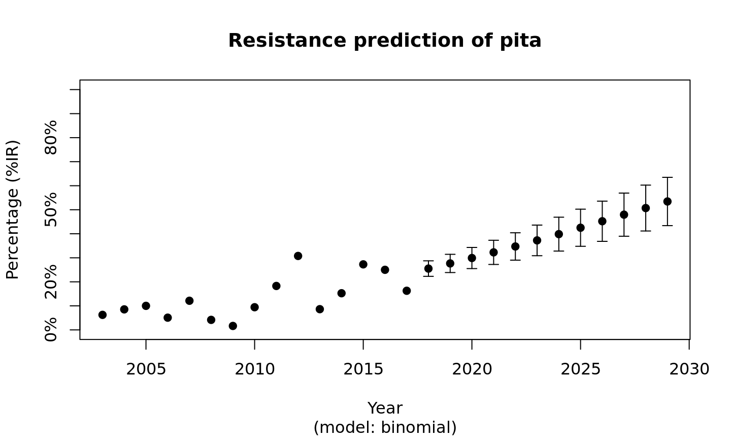
We also support the ggplot2 package with the function ggplot_rsi_predict():
library(ggplot2)
ggplot_rsi_predict(predict_pita)
# Warning: Removed 15 rows containing missing values (geom_errorbar).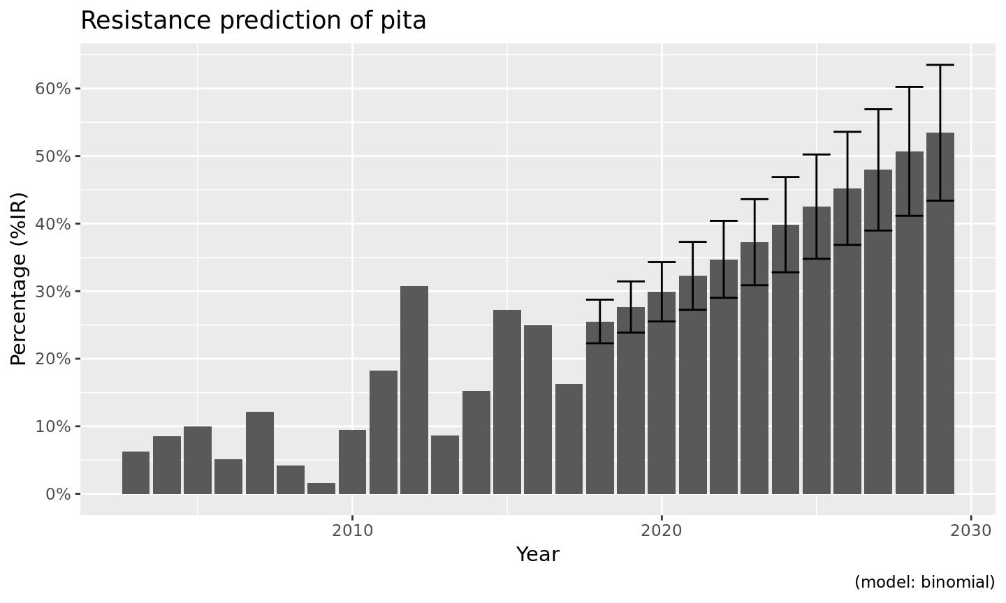
Choosing the right model
Resistance is not easily predicted; if we look at vancomycin resistance in Gram positives, the spread (i.e. standard error) is enormous:
septic_patients %>%
  filter(mo_gramstain(mo) == "Gram positive") %>%
  resistance_predict(col_ab = "vanc", year_min = 2010, info = FALSE) %>%
  plot()
# NOTE: Using column `date` as input for `col_date`.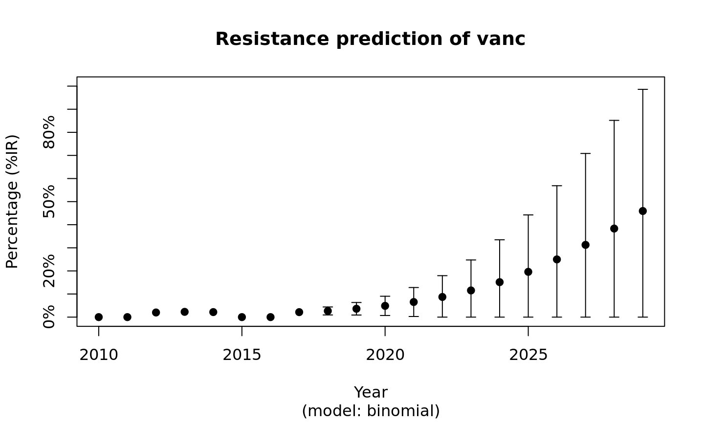
Vancomycin resistance could be 100% in ten years, but might also stay around 0%.
You can define the model with the model parameter. The default model is a generalised linear regression model using a binomial distribution, assuming that a period of zero resistance was followed by a period of increasing resistance leading slowly to more and more resistance.
Valid values are:
| Input values | Function used by R | Type of model |
|---|---|---|
"binomial" or "binom" or "logit"
|
glm(..., family = binomial) |
Generalised linear model with binomial distribution |
"loglin" or "poisson"
|
glm(..., family = poisson) |
Generalised linear model with poisson distribution |
"lin" or "linear"
|
lm() |
Linear model |
For the vancomycin resistance in Gram positive bacteria, a linear model might be more appropriate since no (left half of a) binomial distribution is to be expected based on observed years:
septic_patients %>%
  filter(mo_gramstain(mo) == "Gram positive") %>%
  resistance_predict(col_ab = "vanc", year_min = 2010, info = FALSE, model = "linear") %>%
  plot()
# NOTE: Using column `date` as input for `col_date`.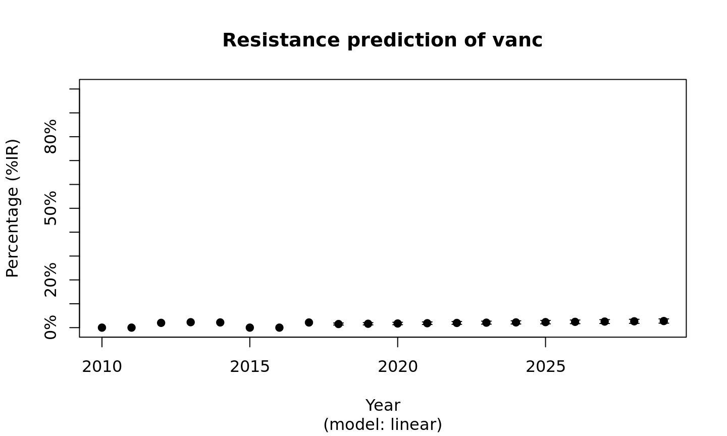
This seems more likely, doesn’t it?