AMR with tidymodels

This page was entirely written by our AMR for R Assistant, a ChatGPT manually-trained model able to answer any question about the AMR package.

Antimicrobial resistance (AMR) is a global health crisis, and understanding resistance patterns is crucial for managing effective treatments. The AMR R package provides robust tools for analysing AMR data, including convenient antimicrobial selector functions like aminoglycosides() and betalactams().

In this post, we will explore how to use the tidymodels framework to predict resistance patterns in the example_isolates dataset in two examples.

This post contains the following examples:

1. Using Antimicrobial Selectors
2. Predicting ESBL Presence Using Raw MICs
3. Predicting AMR Over Time

Example 1: Using Antimicrobial Selectors

By leveraging the power of tidymodels and the AMR package, we’ll build a reproducible machine learning workflow to predict the Gramstain of the microorganism to two important antibiotic classes: aminoglycosides and beta-lactams.

Objective

Our goal is to build a predictive model using the tidymodels framework to determine the Gramstain of the microorganism based on microbial data. We will:

1. Preprocess data using the selector functions aminoglycosides() and betalactams().
2. Define a logistic regression model for prediction.
3. Use a structured tidymodels workflow to preprocess, train, and evaluate the model.

Data Preparation

We begin by loading the required libraries and preparing the example_isolates dataset from the AMR package.

# Load required libraries
library(AMR)          # For AMR data analysis
library(tidymodels)   # For machine learning workflows, and data manipulation (dplyr, tidyr, ...)

Prepare the data:

# Your data could look like this:
example_isolates
#> # A tibble: 2,000 × 46
#>    date       patient   age gender ward     mo           PEN   OXA   FLC   AMX  
#>    <date>     <chr>   <dbl> <chr>  <chr>    <mo>         <sir> <sir> <sir> <sir>
#>  1 2002-01-02 A77334     65 F      Clinical B_ESCHR_COLI   R     NA    NA    NA 
#>  2 2002-01-03 A77334     65 F      Clinical B_ESCHR_COLI   R     NA    NA    NA 
#>  3 2002-01-07 067927     45 F      ICU      B_STPHY_EPDR   R     NA    R     NA 
#>  4 2002-01-07 067927     45 F      ICU      B_STPHY_EPDR   R     NA    R     NA 
#>  5 2002-01-13 067927     45 F      ICU      B_STPHY_EPDR   R     NA    R     NA 
#>  6 2002-01-13 067927     45 F      ICU      B_STPHY_EPDR   R     NA    R     NA 
#>  7 2002-01-14 462729     78 M      Clinical B_STPHY_AURS   R     NA    S     R  
#>  8 2002-01-14 462729     78 M      Clinical B_STPHY_AURS   R     NA    S     R  
#>  9 2002-01-16 067927     45 F      ICU      B_STPHY_EPDR   R     NA    R     NA 
#> 10 2002-01-17 858515     79 F      ICU      B_STPHY_EPDR   R     NA    S     NA 
#> # ℹ 1,990 more rows
#> # ℹ 36 more variables: AMC <sir>, AMP <sir>, TZP <sir>, CZO <sir>, FEP <sir>,
#> #   CXM <sir>, FOX <sir>, CTX <sir>, CAZ <sir>, CRO <sir>, GEN <sir>,
#> #   TOB <sir>, AMK <sir>, KAN <sir>, TMP <sir>, SXT <sir>, NIT <sir>,
#> #   FOS <sir>, LNZ <sir>, CIP <sir>, MFX <sir>, VAN <sir>, TEC <sir>,
#> #   TCY <sir>, TGC <sir>, DOX <sir>, ERY <sir>, CLI <sir>, AZM <sir>,
#> #   IPM <sir>, MEM <sir>, MTR <sir>, CHL <sir>, COL <sir>, MUP <sir>, …

# Select relevant columns for prediction
data <- example_isolates %>%
  # select AB results dynamically
  select(mo, aminoglycosides(), betalactams()) %>%
  # replace NAs with NI (not-interpretable)
   mutate(across(where(is.sir),
                 ~replace_na(.x, "NI")),
          # make factors of SIR columns
          across(where(is.sir),
                 as.integer),
          # get Gramstain of microorganisms
          mo = as.factor(mo_gramstain(mo))) %>%
  # drop NAs - the ones without a Gramstain (fungi, etc.)
  drop_na()
#> ℹ For aminoglycosides() using columns 'GEN' (gentamicin), 'TOB'
#>   (tobramycin), 'AMK' (amikacin), and 'KAN' (kanamycin)
#> ℹ For betalactams() using columns 'PEN' (benzylpenicillin), 'OXA'
#>   (oxacillin), 'FLC' (flucloxacillin), 'AMX' (amoxicillin), 'AMC'
#>   (amoxicillin/clavulanic acid), 'AMP' (ampicillin), 'TZP'
#>   (piperacillin/tazobactam), 'CZO' (cefazolin), 'FEP' (cefepime), 'CXM'
#>   (cefuroxime), 'FOX' (cefoxitin), 'CTX' (cefotaxime), 'CAZ' (ceftazidime),
#>   'CRO' (ceftriaxone), 'IPM' (imipenem), and 'MEM' (meropenem)

Explanation:

• aminoglycosides() and betalactams() dynamically select columns for antimicrobials in these classes.
• drop_na() ensures the model receives complete cases for training.

Defining the Workflow

We now define the tidymodels workflow, which consists of three steps: preprocessing, model specification, and fitting.

1. Preprocessing with a Recipe

We create a recipe to preprocess the data for modelling.

# Define the recipe for data preprocessing
resistance_recipe <- recipe(mo ~ ., data = data) %>%
  step_corr(c(aminoglycosides(), betalactams()), threshold = 0.9)
resistance_recipe
#> 
#> ── Recipe ──────────────────────────────────────────────────────────────────────
#> 
#> ── Inputs
#> Number of variables by role
#> outcome:    1
#> predictor: 20
#> 
#> ── Operations
#> • Correlation filter on: c(aminoglycosides(), betalactams())

For a recipe that includes at least one preprocessing operation, like we have with step_corr(), the necessary parameters can be estimated from a training set using prep():

prep(resistance_recipe)
#> ℹ For aminoglycosides() using columns 'GEN' (gentamicin), 'TOB'
#>   (tobramycin), 'AMK' (amikacin), and 'KAN' (kanamycin)
#> ℹ For betalactams() using columns 'PEN' (benzylpenicillin), 'OXA'
#>   (oxacillin), 'FLC' (flucloxacillin), 'AMX' (amoxicillin), 'AMC'
#>   (amoxicillin/clavulanic acid), 'AMP' (ampicillin), 'TZP'
#>   (piperacillin/tazobactam), 'CZO' (cefazolin), 'FEP' (cefepime), 'CXM'
#>   (cefuroxime), 'FOX' (cefoxitin), 'CTX' (cefotaxime), 'CAZ' (ceftazidime),
#>   'CRO' (ceftriaxone), 'IPM' (imipenem), and 'MEM' (meropenem)
#> 
#> ── Recipe ──────────────────────────────────────────────────────────────────────
#> 
#> ── Inputs
#> Number of variables by role
#> outcome:    1
#> predictor: 20
#> 
#> ── Training information
#> Training data contained 1968 data points and no incomplete rows.
#> 
#> ── Operations
#> • Correlation filter on: AMX CTX | Trained

Explanation:

• recipe(mo ~ ., data = data) will take the mo column as outcome and all other columns as predictors.
• step_corr() removes predictors (i.e., antibiotic columns) that have a higher correlation than 90%.

Notice how the recipe contains just the antimicrobial selector functions - no need to define the columns specifically. In the preparation (retrieved with prep()) we can see that the columns or variables ‘AMX’ and ‘CTX’ were removed as they correlate too much with existing, other variables.

2. Specifying the Model

We define a logistic regression model since resistance prediction is a binary classification task.

# Specify a logistic regression model
logistic_model <- logistic_reg() %>%
  set_engine("glm") # Use the Generalised Linear Model engine
logistic_model
#> Logistic Regression Model Specification (classification)
#> 
#> Computational engine: glm

Explanation:

• logistic_reg() sets up a logistic regression model.
• set_engine("glm") specifies the use of R’s built-in GLM engine.

3. Building the Workflow

We bundle the recipe and model together into a workflow, which organises the entire modelling process.

# Combine the recipe and model into a workflow
resistance_workflow <- workflow() %>%
  add_recipe(resistance_recipe) %>% # Add the preprocessing recipe
  add_model(logistic_model) # Add the logistic regression model
resistance_workflow
#> ══ Workflow ════════════════════════════════════════════════════════════════════
#> Preprocessor: Recipe
#> Model: logistic_reg()
#> 
#> ── Preprocessor ────────────────────────────────────────────────────────────────
#> 1 Recipe Step
#> 
#> • step_corr()
#> 
#> ── Model ───────────────────────────────────────────────────────────────────────
#> Logistic Regression Model Specification (classification)
#> 
#> Computational engine: glm

Training and Evaluating the Model

To train the model, we split the data into training and testing sets. Then, we fit the workflow on the training set and evaluate its performance.

# Split data into training and testing sets
set.seed(123) # For reproducibility
data_split <- initial_split(data, prop = 0.8) # 80% training, 20% testing
training_data <- training(data_split) # Training set
testing_data <- testing(data_split)   # Testing set

# Fit the workflow to the training data
fitted_workflow <- resistance_workflow %>%
  fit(training_data) # Train the model

Explanation:

• initial_split() splits the data into training and testing sets.
• fit() trains the workflow on the training set.

Notice how in fit(), the antimicrobial selector functions are internally called again. For training, these functions are called since they are stored in the recipe.

Next, we evaluate the model on the testing data.

# Make predictions on the testing set
predictions <- fitted_workflow %>%
  predict(testing_data)                # Generate predictions
probabilities <- fitted_workflow %>%
  predict(testing_data, type = "prob") # Generate probabilities

predictions <- predictions %>%
  bind_cols(probabilities) %>%
  bind_cols(testing_data) # Combine with true labels

predictions
#> # A tibble: 394 × 24
#>    .pred_class   `.pred_Gram-negative` `.pred_Gram-positive` mo        GEN   TOB
#>    <fct>                         <dbl>                 <dbl> <fct>   <int> <int>
#>  1 Gram-positive              1.07e- 1              8.93e- 1 Gram-p…     5     5
#>  2 Gram-positive              3.17e- 8              1.00e+ 0 Gram-p…     5     1
#>  3 Gram-negative              9.99e- 1              1.42e- 3 Gram-n…     5     5
#>  4 Gram-positive              2.22e-16              1   e+ 0 Gram-p…     5     5
#>  5 Gram-negative              9.46e- 1              5.42e- 2 Gram-n…     5     5
#>  6 Gram-positive              1.07e- 1              8.93e- 1 Gram-p…     5     5
#>  7 Gram-positive              2.22e-16              1   e+ 0 Gram-p…     1     5
#>  8 Gram-positive              2.22e-16              1   e+ 0 Gram-p…     4     4
#>  9 Gram-negative              1   e+ 0              2.22e-16 Gram-n…     1     1
#> 10 Gram-positive              6.05e-11              1.00e+ 0 Gram-p…     4     4
#> # ℹ 384 more rows
#> # ℹ 18 more variables: AMK <int>, KAN <int>, PEN <int>, OXA <int>, FLC <int>,
#> #   AMX <int>, AMC <int>, AMP <int>, TZP <int>, CZO <int>, FEP <int>,
#> #   CXM <int>, FOX <int>, CTX <int>, CAZ <int>, CRO <int>, IPM <int>, MEM <int>

# Evaluate model performance
metrics <- predictions %>%
  metrics(truth = mo, estimate = .pred_class) # Calculate performance metrics

metrics
#> # A tibble: 2 × 3
#>   .metric  .estimator .estimate
#>   <chr>    <chr>          <dbl>
#> 1 accuracy binary         0.995
#> 2 kap      binary         0.989


# To assess some other model properties, you can make our own `metrics()` function
our_metrics <- metric_set(accuracy, kap, ppv, npv) # add Positive Predictive Value and Negative Predictive Value
metrics2 <- predictions %>%
  our_metrics(truth = mo, estimate = .pred_class) # run again on our `our_metrics()` function

metrics2
#> # A tibble: 4 × 3
#>   .metric  .estimator .estimate
#>   <chr>    <chr>          <dbl>
#> 1 accuracy binary         0.995
#> 2 kap      binary         0.989
#> 3 ppv      binary         0.987
#> 4 npv      binary         1

Explanation:

• predict() generates predictions on the testing set.
• metrics() computes evaluation metrics like accuracy and kappa.

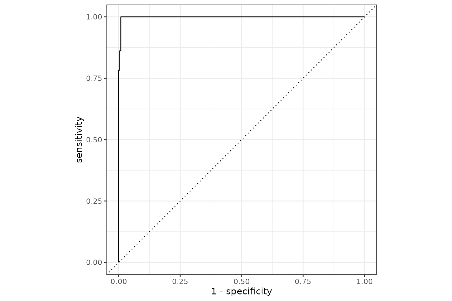
It appears we can predict the Gram stain with a 99.5% accuracy based on AMR results of only aminoglycosides and beta-lactam antibiotics. The ROC curve looks like this:

predictions %>%
  roc_curve(mo, `.pred_Gram-negative`) %>%
  autoplot()

Conclusion

In this post, we demonstrated how to build a machine learning pipeline with the tidymodels framework and the AMR package. By combining selector functions like aminoglycosides() and betalactams() with tidymodels, we efficiently prepared data, trained a model, and evaluated its performance.

This workflow is extensible to other antimicrobial classes and resistance patterns, empowering users to analyse AMR data systematically and reproducibly.

---

Example 2: Predicting ESBL Presence Using Raw MICs

In this second example, we demonstrate how to use <mic> columns directly in tidymodels workflows using AMR-specific recipe steps. This includes a transformation to log2 scale using step_mic_log2(), which prepares MIC values for use in classification models.

This approach and idea formed the basis for the publication DOI: 10.3389/fmicb.2025.1582703 to model the presence of extended-spectrum beta-lactamases (ESBL).

Objective

Our goal is to:

1. Use raw MIC values to predict whether a bacterial isolate produces ESBL.
2. Apply AMR-aware preprocessing in a tidymodels recipe.
3. Train a classification model and evaluate its predictive performance.

Data Preparation

We use the esbl_isolates dataset that comes with the AMR package.

# Load required libraries
library(AMR)
library(tidymodels)

# View the esbl_isolates data set
esbl_isolates
#> # A tibble: 500 × 19
#>    esbl  genus   AMC   AMP   TZP   CXM   FOX   CTX   CAZ   GEN   TOB   TMP   SXT
#>    <lgl> <chr> <mic> <mic> <mic> <mic> <mic> <mic> <mic> <mic> <mic> <mic> <mic>
#>  1 FALSE Esch…    32    32     4    64    64  8.00  8.00     1     1  16.0    20
#>  2 FALSE Esch…    32    32     4    64    64  4.00  8.00     1     1  16.0   320
#>  3 FALSE Esch…     4     2    64     8     4  8.00  0.12    16    16   0.5    20
#>  4 FALSE Kleb…    32    32    16    64    64  8.00  8.00     1     1   0.5    20
#>  5 FALSE Esch…    32    32     4     4     4  0.25  2.00     1     1  16.0   320
#>  6 FALSE Citr…    32    32    16    64    64 64.00 32.00     1     1   0.5    20
#>  7 FALSE Morg…    32    32     4    64    64 16.00  2.00     1     1   0.5    20
#>  8 FALSE Prot…    16    32     4     1     4  8.00  0.12     1     1  16.0   320
#>  9 FALSE Ente…    32    32     8    64    64 32.00  4.00     1     1   0.5    20
#> 10 FALSE Citr…    32    32    32    64    64  8.00 64.00     1     1  16.0   320
#> # ℹ 490 more rows
#> # ℹ 6 more variables: NIT <mic>, FOS <mic>, CIP <mic>, IPM <mic>, MEM <mic>,
#> #   COL <mic>

# Prepare a binary outcome and convert to ordered factor
data <- esbl_isolates %>%
  mutate(esbl = factor(esbl, levels = c(FALSE, TRUE), ordered = TRUE))

Explanation:

• esbl_isolates: Contains MIC test results and ESBL status for each isolate.
• mutate(esbl = ...): Converts the target column to an ordered factor for classification.

Defining the Workflow

1. Preprocessing with a Recipe

We use our step_mic_log2() function to log2-transform MIC values, ensuring that MICs are numeric and properly scaled. All MIC predictors can easily and agnostically selected using the new all_mic_predictors():

# Split into training and testing sets
set.seed(123)
split <- initial_split(data)
training_data <- training(split)
testing_data <- testing(split)

# Define the recipe
mic_recipe <- recipe(esbl ~ ., data = training_data) %>%
  remove_role(genus, old_role = "predictor") %>%  # Remove non-informative variable
  step_mic_log2(all_mic_predictors()) #%>%         # Log2 transform all MIC predictors
 # prep()

mic_recipe
#> 
#> ── Recipe ──────────────────────────────────────────────────────────────────────
#> 
#> ── Inputs
#> Number of variables by role
#> outcome:          1
#> predictor:       17
#> undeclared role:  1
#> 
#> ── Operations
#> • Log2 transformation of MIC columns: all_mic_predictors()

Explanation:

• remove_role(): Removes irrelevant variables like genus.
• step_mic_log2(): Applies log2(as.numeric(...)) to all MIC predictors in one go.
• prep(): Finalises the recipe based on training data.

2. Specifying the Model

We use a simple logistic regression to model ESBL presence, though recent models such as xgboost (link to parsnip manual) could be much more precise.

# Define the model
model <- logistic_reg(mode = "classification") %>%
  set_engine("glm")

model
#> Logistic Regression Model Specification (classification)
#> 
#> Computational engine: glm

Explanation:

• logistic_reg(): Specifies a binary classification model.
• set_engine("glm"): Uses the base R GLM engine.

3. Building the Workflow

# Create workflow
workflow_model <- workflow() %>%
  add_recipe(mic_recipe) %>%
  add_model(model)

workflow_model
#> ══ Workflow ════════════════════════════════════════════════════════════════════
#> Preprocessor: Recipe
#> Model: logistic_reg()
#> 
#> ── Preprocessor ────────────────────────────────────────────────────────────────
#> 1 Recipe Step
#> 
#> • step_mic_log2()
#> 
#> ── Model ───────────────────────────────────────────────────────────────────────
#> Logistic Regression Model Specification (classification)
#> 
#> Computational engine: glm

Training and Evaluating the Model

# Fit the model
fitted <- fit(workflow_model, training_data)

# Generate predictions
predictions <- predict(fitted, testing_data) %>%
  bind_cols(testing_data)

# Evaluate model performance
our_metrics <- metric_set(accuracy, kap, ppv, npv)
metrics <- our_metrics(predictions, truth = esbl, estimate = .pred_class)

metrics
#> # A tibble: 4 × 3
#>   .metric  .estimator .estimate
#>   <chr>    <chr>          <dbl>
#> 1 accuracy binary         0.92 
#> 2 kap      binary         0.840
#> 3 ppv      binary         0.921
#> 4 npv      binary         0.919

Explanation:

• fit(): Trains the model on the processed training data.
• predict(): Produces predictions for unseen test data.
• metric_set(): Allows evaluating multiple classification metrics.

It appears we can predict ESBL gene presence with a positive predictive value (PPV) of 92.1% and a negative predictive value (NPV) of 91.9 using a simplistic logistic regression model.

Visualising Predictions

We can visualise predictions by comparing predicted and actual ESBL status.

library(ggplot2)

ggplot(predictions, aes(x = esbl, fill = .pred_class)) +
  geom_bar(position = "stack") +
  labs(title = "Predicted vs Actual ESBL Status",
       x = "Actual ESBL",
       y = "Count") +
  theme_minimal()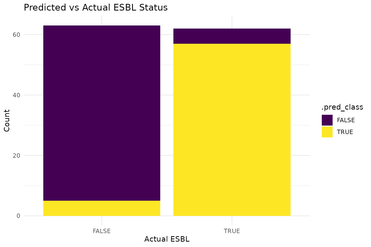

Conclusion

In this example, we showcased how the new AMR-specific recipe steps simplify working with <mic> columns in tidymodels. The step_mic_log2() transformation converts ordered MICs to log2-transformed numerics, improving compatibility with classification models.

This pipeline enables realistic, reproducible, and interpretable modelling of antimicrobial resistance data.

---

Example 3: Predicting AMR Over Time

In this third example, we aim to predict antimicrobial resistance (AMR) trends over time using tidymodels. We will model resistance to three antibiotics (amoxicillin AMX, amoxicillin-clavulanic acid AMC, and ciprofloxacin CIP), based on historical data grouped by year and hospital ward.

Objective

Our goal is to:

1. Prepare the dataset by aggregating resistance data over time.
2. Define a regression model to predict AMR trends.
3. Use tidymodels to preprocess, train, and evaluate the model.

Data Preparation

We start by transforming the example_isolates dataset into a structured time-series format.

# Load required libraries
library(AMR)
library(tidymodels)

# Transform dataset
data_time <- example_isolates %>%
  top_n_microorganisms(n = 10) %>% # Filter on the top #10 species
  mutate(year = as.integer(format(date, "%Y")),  # Extract year from date
         gramstain = mo_gramstain(mo)) %>% # Get taxonomic names
  group_by(year, gramstain) %>%
  summarise(across(c(AMX, AMC, CIP), 
                   function(x) resistance(x, minimum = 0),
                   .names = "res_{.col}"), 
            .groups = "drop") %>% 
  filter(!is.na(res_AMX) & !is.na(res_AMC) & !is.na(res_CIP)) # Drop missing values
#> ℹ Using column 'mo' as input for col_mo.

data_time
#> # A tibble: 32 × 5
#>     year gramstain     res_AMX res_AMC res_CIP
#>    <int> <chr>           <dbl>   <dbl>   <dbl>
#>  1  2002 Gram-negative   1      0.105   0.0606
#>  2  2002 Gram-positive   0.838  0.182   0.162 
#>  3  2003 Gram-negative   1      0.0714  0     
#>  4  2003 Gram-positive   0.714  0.244   0.154 
#>  5  2004 Gram-negative   0.464  0.0938  0     
#>  6  2004 Gram-positive   0.849  0.299   0.244 
#>  7  2005 Gram-negative   0.412  0.132   0.0588
#>  8  2005 Gram-positive   0.882  0.382   0.154 
#>  9  2006 Gram-negative   0.379  0       0.1   
#> 10  2006 Gram-positive   0.778  0.333   0.353 
#> # ℹ 22 more rows

Explanation:

• mo_name(mo): Converts microbial codes into proper species names.
• resistance(): Converts AMR results into numeric values (proportion of resistant isolates).
• group_by(year, ward, species): Aggregates resistance rates by year and ward.

Defining the Workflow

We now define the modelling workflow, which consists of a preprocessing step, a model specification, and the fitting process.

1. Preprocessing with a Recipe

# Define the recipe
resistance_recipe_time <- recipe(res_AMX ~ year + gramstain, data = data_time) %>%
  step_dummy(gramstain, one_hot = TRUE) %>%  # Convert categorical to numerical
  step_normalize(year) %>%  # Normalise year for better model performance
  step_nzv(all_predictors())  # Remove near-zero variance predictors

resistance_recipe_time
#> 
#> ── Recipe ──────────────────────────────────────────────────────────────────────
#> 
#> ── Inputs
#> Number of variables by role
#> outcome:   1
#> predictor: 2
#> 
#> ── Operations
#> • Dummy variables from: gramstain
#> • Centering and scaling for: year
#> • Sparse, unbalanced variable filter on: all_predictors()

Explanation:

• step_dummy(): Encodes categorical variables (ward, species) as numerical indicators.
• step_normalize(): Normalises the year variable.
• step_nzv(): Removes near-zero variance predictors.

2. Specifying the Model

We use a linear regression model to predict resistance trends.

# Define the linear regression model
lm_model <- linear_reg() %>%
  set_engine("lm") # Use linear regression

lm_model
#> Linear Regression Model Specification (regression)
#> 
#> Computational engine: lm

Explanation:

• linear_reg(): Defines a linear regression model.
• set_engine("lm"): Uses R’s built-in linear regression engine.

3. Building the Workflow

We combine the preprocessing recipe and model into a workflow.

# Create workflow
resistance_workflow_time <- workflow() %>%
  add_recipe(resistance_recipe_time) %>%
  add_model(lm_model)

resistance_workflow_time
#> ══ Workflow ════════════════════════════════════════════════════════════════════
#> Preprocessor: Recipe
#> Model: linear_reg()
#> 
#> ── Preprocessor ────────────────────────────────────────────────────────────────
#> 3 Recipe Steps
#> 
#> • step_dummy()
#> • step_normalize()
#> • step_nzv()
#> 
#> ── Model ───────────────────────────────────────────────────────────────────────
#> Linear Regression Model Specification (regression)
#> 
#> Computational engine: lm

Training and Evaluating the Model

We split the data into training and testing sets, fit the model, and evaluate performance.

# Split the data
set.seed(123)
data_split_time <- initial_split(data_time, prop = 0.8)
train_time <- training(data_split_time)
test_time <- testing(data_split_time)

# Train the model
fitted_workflow_time <- resistance_workflow_time %>%
  fit(train_time)

# Make predictions
predictions_time <- fitted_workflow_time %>%
  predict(test_time) %>%
  bind_cols(test_time) 

# Evaluate model
metrics_time <- predictions_time %>%
  metrics(truth = res_AMX, estimate = .pred)

metrics_time
#> # A tibble: 3 × 3
#>   .metric .estimator .estimate
#>   <chr>   <chr>          <dbl>
#> 1 rmse    standard      0.0774
#> 2 rsq     standard      0.711 
#> 3 mae     standard      0.0704

Explanation:

• initial_split(): Splits data into training and testing sets.
• fit(): Trains the workflow.
• predict(): Generates resistance predictions.
• metrics(): Evaluates model performance.

Visualising Predictions

We plot resistance trends over time for amoxicillin.

library(ggplot2)

# Plot actual vs predicted resistance over time
ggplot(predictions_time, aes(x = year)) +
  geom_point(aes(y = res_AMX, color = "Actual")) +
  geom_line(aes(y = .pred, color = "Predicted")) +
  labs(title = "Predicted vs Actual AMX Resistance Over Time",
       x = "Year",
       y = "Resistance Proportion") +
  theme_minimal()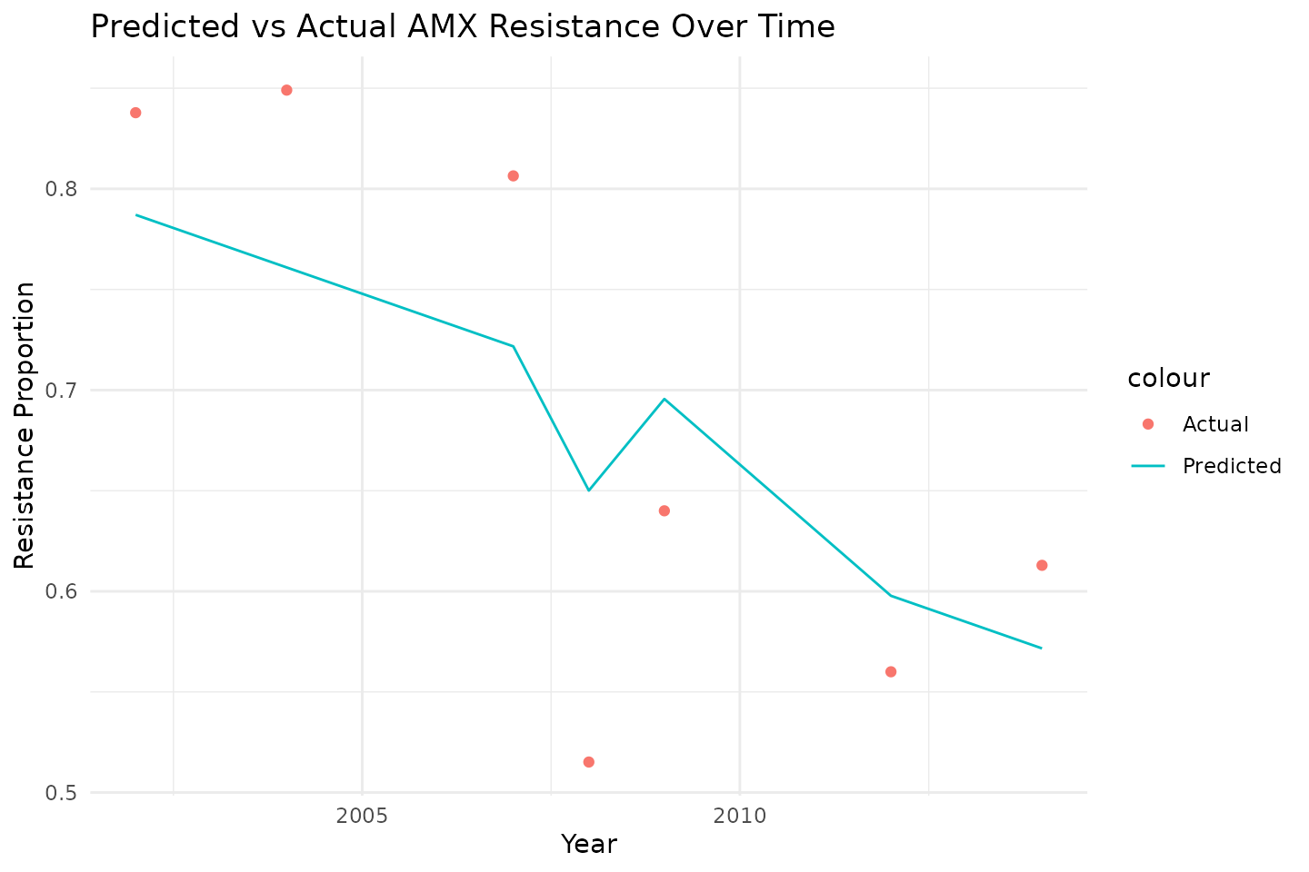

Additionally, we can visualise resistance trends in ggplot2 and directly add linear models there:

ggplot(data_time, aes(x = year, y = res_AMX, color = gramstain)) +
  geom_line() +
  labs(title = "AMX Resistance Trends",
       x = "Year",
       y = "Resistance Proportion") +
  # add a linear model directly in ggplot2:
  geom_smooth(method = "lm",
              formula = y ~ x,
              alpha = 0.25) +
  theme_minimal()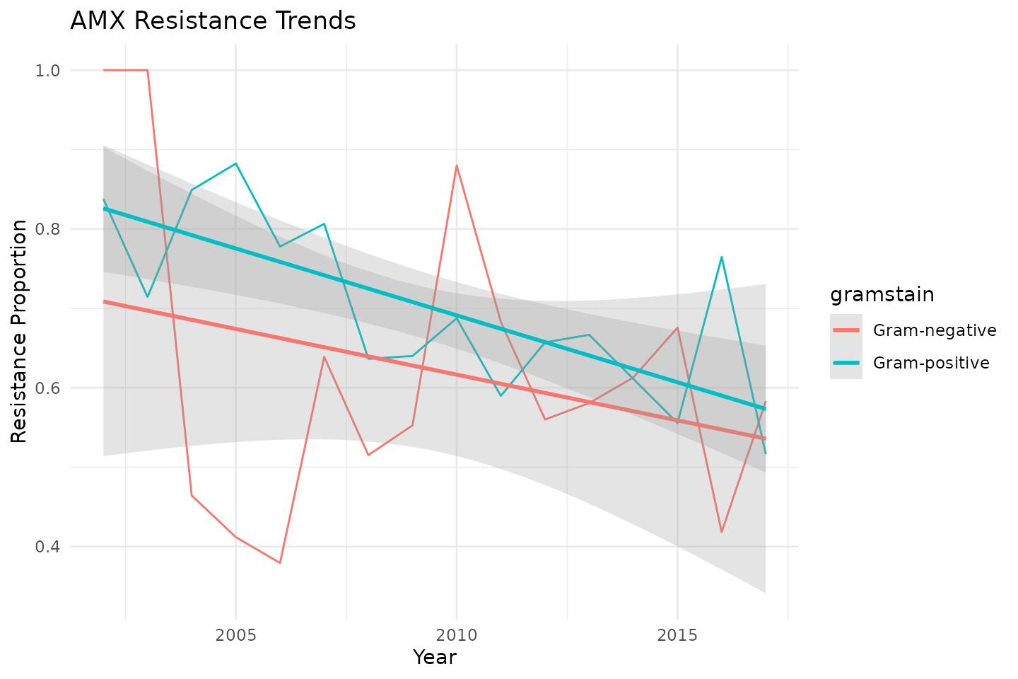

Conclusion

In this example, we demonstrated how to analyze AMR trends over time using tidymodels. By aggregating resistance rates by year and hospital ward, we built a predictive model to track changes in resistance to amoxicillin (AMX), amoxicillin-clavulanic acid (AMC), and ciprofloxacin (CIP).

This method can be extended to other antibiotics and resistance patterns, providing valuable insights into AMR dynamics in healthcare settings.