Note: values on this page will change with every website update since they are based on randomly created values and the page was written in R Markdown. However, the methodology remains unchanged. This page was generated on 23 June 2026.
Introduction
Conducting AMR data analysis unfortunately requires in-depth knowledge from different scientific fields, which makes it hard to do right. At least, it requires:
- Good questions (always start with those!) and reliable data
- A thorough understanding of (clinical) epidemiology, to understand the clinical and epidemiological relevance and possible bias of results
- A thorough understanding of (clinical) microbiology/infectious diseases, to understand which microorganisms are causal to which infections and the implications of pharmaceutical treatment, as well as understanding intrinsic and acquired microbial resistance
- Experience with data analysis with microbiological tests and their results, to understand the determination and limitations of MIC values and their interpretations to SIR values
- Availability of the biological taxonomy of microorganisms and probably normalisation factors for pharmaceuticals, such as defined daily doses (DDD)
- Available (inter-)national guidelines, and profound methods to apply them
Of course, we cannot instantly provide you with knowledge and
experience. But with this AMR package, we aimed at
providing (1) tools to simplify antimicrobial resistance data cleaning,
transformation and analysis, (2) methods to easily incorporate
international guidelines and (3) scientifically reliable reference data,
including the requirements mentioned above.
The AMR package enables standardised and reproducible
AMR data analysis, with the application of evidence-based rules,
determination of first isolates, translation of various codes for
microorganisms and antimicrobial drugs, determination of (multi-drug)
resistant microorganisms, and calculation of antimicrobial resistance,
prevalence and future trends.
Preparation
For this tutorial, we will create fake demonstration data to work with.
You can skip to Cleaning the data if you already have your own data ready. If you start your analysis, try to make the structure of your data generally look like this:
| date | patient_id | mo | AMX | CIP |
|---|---|---|---|---|
| 2026-06-23 | abcd | Escherichia coli | S | S |
| 2026-06-23 | abcd | Escherichia coli | S | R |
| 2026-06-23 | efgh | Escherichia coli | R | S |
Needed R packages
As with many uses in R, we need some additional packages for AMR data
analysis. Our package works closely together with the tidyverse packages dplyr and ggplot2 by
RStudio. The tidyverse tremendously improves the way we conduct data
science - it allows for a very natural way of writing syntaxes and
creating beautiful plots in R.
We will also use the cleaner package, that can be used
for cleaning data and creating frequency tables.
library(dplyr)
library(ggplot2)
library(AMR)

# (if not yet installed, install with:)
# install.packages(c("dplyr", "ggplot2", "AMR"))
The AMR package contains a data set
example_isolates_unclean, which might look data that users
have extracted from their laboratory systems:
example_isolates_unclean
#> # A tibble: 3,000 × 8
#>    patient_id hospital date       bacteria      AMX   AMC   CIP   GEN
#>    <chr>      <chr>    <date>     <chr>         <chr> <chr> <chr> <chr>
#>  1 J3         A        2012-11-21 E. coli       R     I     S     S
#>  2 R7         A        2018-04-03 K. pneumoniae R     I     S     S
#>  3 P3         A        2014-09-19 E. coli       R     S     S     S
#>  4 P10        A        2015-12-10 E. coli       S     I     S     S
#>  5 B7         A        2015-03-02 E. coli       S     S     S     S
#>  6 W3         A        2018-03-31 S. aureus     R     S     R     S
#>  7 J8         A        2016-06-14 E. coli       R     S     S     S
#>  8 M3         A        2015-10-25 E. coli       R     S     S     S
#>  9 J3         A        2019-06-19 E. coli       S     S     S     S
#> 10 G6         A        2015-04-27 S. aureus     S     S     S     S
#> # ℹ 2,990 more rows

# we will use 'our_data' as the data set name for this tutorial
our_data <- example_isolates_unclean
For AMR data analysis, we would like the microorganism column to contain valid, up-to-date taxonomy, and the antibiotic columns to be cleaned as SIR values as well.
Taxonomy of microorganisms
With as.mo(), users can transform arbitrary
microorganism names or codes to current taxonomy. The AMR
package contains up-to-date taxonomic data. To be specific, currently
included data were retrieved on 07 May 2026.
The codes of the AMR packages that come from as.mo() are
short, but still human readable. More importantly, as.mo()
supports all kinds of input:
as.mo("Klebsiella pneumoniae")
#> Class <mo>
#> [1] B_KLBSL_PNMN
as.mo("K. pneumoniae")
#> Class <mo>
#> [1] B_KLBSL_PNMN
as.mo("KLEPNE")
#> Class <mo>
#> [1] B_KLBSL_PNMN
as.mo("KLPN")
#> Class <mo>
#> [1] B_KLBSL_PNMN
The first character in above codes denote their taxonomic kingdom, such as Bacteria (B), Fungi (F), and Protozoa (P).
The AMR package also contain functions to directly
retrieve taxonomic properties, such as the name, genus, species, family,
order, and even Gram-stain. They all start with mo_ and
they use as.mo() internally, so that still any arbitrary
user input can be used:
mo_family("K. pneumoniae")
#> [1] "Enterobacteriaceae"
mo_genus("K. pneumoniae")
#> [1] "Klebsiella"
mo_species("K. pneumoniae")
#> [1] "pneumoniae"

mo_gramstain("Klebsiella pneumoniae")
#> [1] "Gram-negative"

mo_ref("K. pneumoniae")
#> [1] "Trevisan, 1887"

mo_snomed("K. pneumoniae")
#> [[1]]
#> [1] "1098101000112102" "446870005"        "1098201000112108" "409801009"
#> [5] "56415008"         "714315002"        "713926009"
Now we can thus clean our data:
our_data$bacteria <- as.mo(our_data$bacteria, info = TRUE)
#> ℹ Retrieved values from the `microorganisms.codes` data set for "ESCCOL",
#>   "KLEPNE", "STAAUR", and "STRPNE".
#> ℹ Microorganism translation was uncertain for four microorganisms. Run
#>   `mo_uncertainties()` to review these uncertainties, or use
#>   `add_custom_microorganisms()` to add custom entries.
Apparently, there was some uncertainty about the translation to taxonomic codes. Let’s check this:
mo_uncertainties()
#> Matching scores are based on the resemblance between the input and the full
#> taxonomic name, and the pathogenicity in humans. See `mo_matching_score()`.
#> Colour keys:  0.000-0.549  0.550-0.649  0.650-0.749  0.750-1.000
#> -------------------------------------------------------------------------------
#> "E. coli" -> Escherichia coli (B_ESCHR_COLI, 0.688)
#> Also matched: Enterococcus crotali (0.650), Escherichia coli coli (0.643),
#> Escherichia coli expressing (0.611), Enterobacter cowanii (0.600), Enterococcus
#> columbae (0.595), Enterococcus camelliae (0.591), Enterococcus casseliflavus
#> (0.577), Enterobacter cloacae cloacae (0.571), Enterobacter cloacae complex
#> (0.571), and Enterobacter cloacae dissolvens (0.565)
#> -------------------------------------------------------------------------------
#> "K. pneumoniae" -> Klebsiella pneumoniae (B_KLBSL_PNMN, 0.786)
#> Also matched: Klebsiella pneumoniae complex (0.707), Klebsiella pneumoniae
#> ozaenae (0.707), Klebsiella pneumoniae pneumoniae (0.688), Klebsiella
#> pneumoniae rhinoscleromatis (0.658), Klebsiella pasteurii (0.500), Klebsiella
#> planticola (0.500), Kosakonia pseudosacchari (0.471), Kaistella palustris
#> (0.435), Kingella potus (0.435), and Kocuria palustris (0.435)
#> -------------------------------------------------------------------------------
#> "S. aureus" -> Staphylococcus aureus (B_STPHY_AURS, 0.690)
#> Also matched: Staphylococcus aureus aureus (0.643), Staphylococcus argenteus
#> (0.625), Staphylococcus aureus anaerobius (0.625), Streptomyces aureus (0.618),
#> Staphylococcus auricularis (0.615), Streptomyces azureus (0.609), Salmonella
#> Aurelianis (0.595), Salmonella Aarhus (0.588), Salmonella Amounderness (0.587),
#> and Staphylococcus argensis (0.587)
#> -------------------------------------------------------------------------------
#> "S. pneumoniae" -> Streptococcus pneumoniae (B_STRPT_PNMN, 0.750)
#> Also matched: Streptococcus parapneumoniae (0.714), Streptococcus
#> pseudopneumoniae (0.700), Serratia proteamaculans quinivorans (0.557),
#> Streptococcus phocae salmonis (0.552), Serratia proteamaculans quinovora
#> (0.545), Sphingomonas piscinae (0.538), Streptococcus pseudoporcinus (0.536),
#> Staphylococcus piscifermentans (0.533), Staphylococcus pseudintermedius
#> (0.532), and Serratia proteamaculans proteamaculans (0.526)
#> ℹ Only the first 10 other matches of each record are shown. Run ``
#>   `print(mo_uncertainties(), n = ...)` `` to view more entries, or save
#>   `mo_uncertainties()` to an object.
That’s all good.
Antibiotic results
The column with antibiotic test results must also be cleaned. The
AMR package comes with three new data types to work with
such test results: mic for minimal inhibitory
concentrations (MIC), disk for disk diffusion diameters,
and sir for SIR data that have been interpreted already.
This package can also determine SIR values based on MIC or disk
diffusion values, read more about that on the as.sir()
page.
For now, we will just clean the SIR columns in our data using dplyr:
# method 1, be explicit about the columns:
our_data <- our_data %>%
  mutate_at(vars(AMX:GEN), as.sir)

# method 2, let the AMR package determine the eligible columns
our_data <- our_data %>%
  mutate_if(is_sir_eligible, as.sir)

# result:
our_data
#> # A tibble: 3,000 × 8
#>    patient_id hospital date       bacteria     AMX   AMC   CIP   GEN
#>    <chr>      <chr>    <date>     <mo>         <sir> <sir> <sir> <sir>
#>  1 J3         A        2012-11-21 B_ESCHR_COLI   R     I     S     S
#>  2 R7         A        2018-04-03 B_KLBSL_PNMN   R     I     S     S
#>  3 P3         A        2014-09-19 B_ESCHR_COLI   R     S     S     S
#>  4 P10        A        2015-12-10 B_ESCHR_COLI   S     I     S     S
#>  5 B7         A        2015-03-02 B_ESCHR_COLI   S     S     S     S
#>  6 W3         A        2018-03-31 B_STPHY_AURS   R     S     R     S
#>  7 J8         A        2016-06-14 B_ESCHR_COLI   R     S     S     S
#>  8 M3         A        2015-10-25 B_ESCHR_COLI   R     S     S     S
#>  9 J3         A        2019-06-19 B_ESCHR_COLI   S     S     S     S
#> 10 G6         A        2015-04-27 B_STPHY_AURS   S     S     S     S
#> # ℹ 2,990 more rows
This is basically it for the cleaning, time to start the data inclusion.
First isolates
We need to know which isolates we can actually use for analysis without repetition bias.
To conduct an analysis of antimicrobial resistance, you must only include the first isolate of every patient per episode (Hindler et al., Clin Infect Dis. 2007). If you would not do this, you could easily get an overestimate or underestimate of the resistance of an antibiotic. Imagine that a patient was admitted with an MRSA and that it was found in 5 different blood cultures the following weeks (yes, some countries like the Netherlands have these blood drawing policies). The resistance percentage of oxacillin of all isolates would be overestimated, because you included this MRSA more than once. It would clearly be selection bias.
The Clinical and Laboratory Standards Institute (CLSI) appoints this as follows:
(…) When preparing a cumulative antibiogram to guide clinical decisions about empirical antimicrobial therapy of initial infections, only the first isolate of a given species per patient, per analysis period (eg, one year) should be included, irrespective of body site, antimicrobial susceptibility profile, or other phenotypical characteristics (eg, biotype). The first isolate is easily identified, and cumulative antimicrobial susceptibility test data prepared using the first isolate are generally comparable to cumulative antimicrobial susceptibility test data calculated by other methods, providing duplicate isolates are excluded.
M39-A4 Analysis and Presentation of Cumulative Antimicrobial Susceptibility Test Data, 4th Edition. CLSI, 2014. Chapter 6.4
This AMR package includes this methodology with the
first_isolate() function and is able to apply the four
different methods as defined by Hindler
et al. in 2007: phenotype-based, episode-based,
patient-based, isolate-based. The right method depends on your goals and
analysis, but the default phenotype-based method is in any case the
method to properly correct for most duplicate isolates. Read more about
the methods on the first_isolate() page.
The outcome of the function can easily be added to our data:
our_data <- our_data %>%
  mutate(first = first_isolate(info = TRUE))
#> ℹ Determining first isolates using an episode length of 365 days
#> ℹ Using column bacteria as input for `col_mo`.
#> ℹ Column first is SIR eligible (despite only having empty values), since it
#>   seems to be cefozopran (ZOP)
#> ℹ Using column date as input for `col_date`.
#> ℹ Using column patient_id as input for `col_patient_id`.
#> ℹ Basing inclusion on all antimicrobial results, using a points threshold of 2
#> => Found 2,724 'phenotype-based' first isolates (90.8% of total where a
#> microbial ID was available)
So only 91% is suitable for resistance analysis! We can now filter on
it with the filter() function, also from the
dplyr package:
For future use, the above two syntaxes can be shortened:
our_data_1st <- our_data %>%
  filter_first_isolate()
So we end up with 2 724 isolates for analysis. Now our data looks like:
our_data_1st
#> # A tibble: 2,724 × 9
#>    patient_id hospital date       bacteria     AMX   AMC   CIP   GEN   first
#>    <chr>      <chr>    <date>     <mo>         <sir> <sir> <sir> <sir> <lgl>
#>  1 J3         A        2012-11-21 B_ESCHR_COLI   R     I     S     S   TRUE
#>  2 R7         A        2018-04-03 B_KLBSL_PNMN   R     I     S     S   TRUE
#>  3 P3         A        2014-09-19 B_ESCHR_COLI   R     S     S     S   TRUE
#>  4 P10        A        2015-12-10 B_ESCHR_COLI   S     I     S     S   TRUE
#>  5 B7         A        2015-03-02 B_ESCHR_COLI   S     S     S     S   TRUE
#>  6 W3         A        2018-03-31 B_STPHY_AURS   R     S     R     S   TRUE
#>  7 M3         A        2015-10-25 B_ESCHR_COLI   R     S     S     S   TRUE
#>  8 J3         A        2019-06-19 B_ESCHR_COLI   S     S     S     S   TRUE
#>  9 G6         A        2015-04-27 B_STPHY_AURS   S     S     S     S   TRUE
#> 10 P4         A        2011-06-21 B_ESCHR_COLI   S     S     S     S   TRUE
#> # ℹ 2,714 more rows
Time for the analysis.
Analysing the data
The base R summary() function gives a good first
impression, as it comes with support for the new mo and
sir classes that we now have in our data set:
summary(our_data_1st)
#>      patient_id        hospital         date              bacteria
#>  Length   :2724   Length   :2724   Min.   :2011-01-01   Class :mo
#>  N.unique : 260   N.unique :   3   1st Qu.:2013-04-07   <NA>  :0
#>  N.blank  :   0   N.blank  :   0   Median :2015-06-03   Unique:4
#>  Min.nchar:   2   Min.nchar:   1   Mean   :2015-06-09   #1    :B_ESCHR_COLI
#>  Max.nchar:   3   Max.nchar:   1   3rd Qu.:2017-08-11   #2    :B_STPHY_AURS
#>                                    Max.   :2019-12-27   #3    :B_STRPT_PNMN
#>     AMX                    AMC                    CIP
#>  Class:sir              Class:sir              Class:sir
#>  %S   :41.6% (n=1133)   %S   :52.6% (n=1432)   %S   :52.5% (n=1431)
#>  %SDD : 0.0% (n=0)      %SDD : 0.0% (n=0)      %SDD : 0.0% (n=0)
#>  %I   :16.4% (n=446)    %I   :12.2% (n=333)    %I   : 6.5% (n=176)
#>  %R   :42.0% (n=1145)   %R   :35.2% (n=959)    %R   :41.0% (n=1117)
#>  %NI  : 0.0% (n=0)      %NI  : 0.0% (n=0)      %NI  : 0.0% (n=0)
#>     GEN                  first
#>  Class:sir              Mode:logical
#>  %S   :61.0% (n=1661)   TRUE:2724
#>  %SDD : 0.0% (n=0)
#>  %I   : 3.0% (n=82)
#>  %R   :36.0% (n=981)
#>  %NI  : 0.0% (n=0)

glimpse(our_data_1st)
#> Rows: 2,724
#> Columns: 9
#> $ patient_id <chr> "J3", "R7", "P3", "P10", "B7", "W3", "M3", "J3", "G6", "P4"…
#> $ hospital   <chr> "A", "A", "A", "A", "A", "A", "A", "A", "A", "A", "A", "A",…
#> $ date       <date> 2012-11-21, 2018-04-03, 2014-09-19, 2015-12-10, 2015-03-02…
#> $ bacteria   <mo> "B_ESCHR_COLI", "B_KLBSL_PNMN", "B_ESCHR_COLI", "B_ESCHR_COL…
#> $ AMX        <sir> R, R, R, S, S, R, R, S, S, S, S, R, S, S, R, R, R, R, S, R,…
#> $ AMC        <sir> I, I, S, I, S, S, S, S, S, S, S, S, S, S, S, S, S, R, S, S,…
#> $ CIP        <sir> S, S, S, S, S, R, S, S, S, S, S, S, S, S, S, S, S, S, S, S,…
#> $ GEN        <sir> S, S, S, S, S, S, S, S, S, S, S, R, S, S, S, S, S, S, S, S,…
#> $ first      <lgl> TRUE, TRUE, TRUE, TRUE, TRUE, TRUE, TRUE, TRUE, TRUE, TRUE,…

# number of unique values per column:
sapply(our_data_1st, n_distinct)
#> patient_id   hospital       date   bacteria        AMX        AMC        CIP
#>        260          3       1854          4          3          3          3
#>        GEN      first
#>          3          1
Availability of species
To just get an idea how the species are distributed, create a
frequency table with count() based on the name of the
microorganisms:
our_data %>%
  count(mo_name(bacteria), sort = TRUE)
#> # A tibble: 4 × 2
#>   `mo_name(bacteria)`          n
#>   <chr>                    <int>
#> 1 Escherichia coli          1518
#> 2 Staphylococcus aureus      730
#> 3 Streptococcus pneumoniae   426
#> 4 Klebsiella pneumoniae      326

our_data_1st %>%
  count(mo_name(bacteria), sort = TRUE)
#> # A tibble: 4 × 2
#>   `mo_name(bacteria)`          n
#>   <chr>                    <int>
#> 1 Escherichia coli          1321
#> 2 Staphylococcus aureus      682
#> 3 Streptococcus pneumoniae   402
#> 4 Klebsiella pneumoniae      319
Select and filter with antibiotic selectors
Using so-called antibiotic class selectors, you can select or filter columns based on the antibiotic class that your antibiotic results are in:
our_data_1st %>%
  select(date, aminoglycosides())
#> ℹ For `aminoglycosides()` using column GEN
#> (gentamicin)
#> # A tibble: 2,724 × 2
#>    date       GEN
#>    <date>     <sir>
#>  1 2012-11-21   S
#>  2 2018-04-03   S
#>  3 2014-09-19   S
#>  4 2015-12-10   S
#>  5 2015-03-02   S
#>  6 2018-03-31   S
#>  7 2015-10-25   S
#>  8 2019-06-19   S
#>  9 2015-04-27   S
#> 10 2011-06-21   S
#> # ℹ 2,714 more rows

our_data_1st %>%
  select(bacteria, betalactams())
#> ℹ For `betalactams()` using columns AMX (amoxicillin) and AMC
#>   (amoxicillin/clavulanic acid)
#> # A tibble: 2,724 × 3
#>    bacteria     AMX   AMC
#>    <mo>         <sir> <sir>
#>  1 B_ESCHR_COLI   R     I
#>  2 B_KLBSL_PNMN   R     I
#>  3 B_ESCHR_COLI   R     S
#>  4 B_ESCHR_COLI   S     I
#>  5 B_ESCHR_COLI   S     S
#>  6 B_STPHY_AURS   R     S
#>  7 B_ESCHR_COLI   R     S
#>  8 B_ESCHR_COLI   S     S
#>  9 B_STPHY_AURS   S     S
#> 10 B_ESCHR_COLI   S     S
#> # ℹ 2,714 more rows

our_data_1st %>%
  select(bacteria, where(is.sir))
#> # A tibble: 2,724 × 5
#>    bacteria     AMX   AMC   CIP   GEN
#>    <mo>         <sir> <sir> <sir> <sir>
#>  1 B_ESCHR_COLI   R     I     S     S
#>  2 B_KLBSL_PNMN   R     I     S     S
#>  3 B_ESCHR_COLI   R     S     S     S
#>  4 B_ESCHR_COLI   S     I     S     S
#>  5 B_ESCHR_COLI   S     S     S     S
#>  6 B_STPHY_AURS   R     S     R     S
#>  7 B_ESCHR_COLI   R     S     S     S
#>  8 B_ESCHR_COLI   S     S     S     S
#>  9 B_STPHY_AURS   S     S     S     S
#> 10 B_ESCHR_COLI   S     S     S     S
#> # ℹ 2,714 more rows

# filtering using AB selectors is also possible:
our_data_1st %>%
  filter(any(aminoglycosides() == "R"))
#> ℹ For `aminoglycosides()` using column GEN
#> (gentamicin)
#> # A tibble: 981 × 9
#>    patient_id hospital date       bacteria     AMX   AMC   CIP   GEN   first
#>    <chr>      <chr>    <date>     <mo>         <sir> <sir> <sir> <sir> <lgl>
#>  1 J5         A        2017-12-25 B_STRPT_PNMN   R     S     S     R   TRUE
#>  2 X1         A        2017-07-04 B_STPHY_AURS   R     S     S     R   TRUE
#>  3 B3         A        2016-07-24 B_ESCHR_COLI   S     S     S     R   TRUE
#>  4 V7         A        2012-04-03 B_ESCHR_COLI   S     S     S     R   TRUE
#>  5 C9         A        2017-03-23 B_ESCHR_COLI   S     S     S     R   TRUE
#>  6 R1         A        2018-06-10 B_STPHY_AURS   S     S     S     R   TRUE
#>  7 S2         A        2013-07-19 B_STRPT_PNMN   S     S     S     R   TRUE
#>  8 P5         A        2019-03-09 B_STPHY_AURS   S     S     S     R   TRUE
#>  9 Q8         A        2019-08-10 B_STPHY_AURS   S     S     S     R   TRUE
#> 10 K5         A        2013-03-15 B_STRPT_PNMN   S     S     S     R   TRUE
#> # ℹ 971 more rows

our_data_1st %>%
  filter(all(betalactams() == "R"))
#> ℹ For `betalactams()` using columns AMX (amoxicillin) and AMC
#>   (amoxicillin/clavulanic acid)
#> # A tibble: 462 × 9
#>    patient_id hospital date       bacteria     AMX   AMC   CIP   GEN   first
#>    <chr>      <chr>    <date>     <mo>         <sir> <sir> <sir> <sir> <lgl>
#>  1 M7         A        2013-07-22 B_STRPT_PNMN   R     R     S     S   TRUE
#>  2 R10        A        2013-12-20 B_STPHY_AURS   R     R     S     S   TRUE
#>  3 R7         A        2015-10-25 B_STPHY_AURS   R     R     S     S   TRUE
#>  4 R8         A        2019-10-25 B_STPHY_AURS   R     R     S     S   TRUE
#>  5 B6         A        2016-11-20 B_ESCHR_COLI   R     R     R     R   TRUE
#>  6 I7         A        2015-08-19 B_ESCHR_COLI   R     R     S     S   TRUE
#>  7 N3         A        2014-12-29 B_STRPT_PNMN   R     R     R     S   TRUE
#>  8 Q2         A        2019-09-22 B_ESCHR_COLI   R     R     S     S   TRUE
#>  9 X7         A        2011-03-20 B_ESCHR_COLI   R     R     S     R   TRUE
#> 10 V1         A        2018-08-07 B_STPHY_AURS   R     R     S     S   TRUE
#> # ℹ 452 more rows

# even works in base R (since R 3.0):
our_data_1st[all(betalactams() == "R"), ]
#> ℹ For `betalactams()` using columns AMX (amoxicillin) and AMC
#>   (amoxicillin/clavulanic acid)
#> # A tibble: 462 × 9
#>    patient_id hospital date       bacteria     AMX   AMC   CIP   GEN   first
#>    <chr>      <chr>    <date>     <mo>         <sir> <sir> <sir> <sir> <lgl>
#>  1 M7         A        2013-07-22 B_STRPT_PNMN   R     R     S     S   TRUE
#>  2 R10        A        2013-12-20 B_STPHY_AURS   R     R     S     S   TRUE
#>  3 R7         A        2015-10-25 B_STPHY_AURS   R     R     S     S   TRUE
#>  4 R8         A        2019-10-25 B_STPHY_AURS   R     R     S     S   TRUE
#>  5 B6         A        2016-11-20 B_ESCHR_COLI   R     R     R     R   TRUE
#>  6 I7         A        2015-08-19 B_ESCHR_COLI   R     R     S     S   TRUE
#>  7 N3         A        2014-12-29 B_STRPT_PNMN   R     R     R     S   TRUE
#>  8 Q2         A        2019-09-22 B_ESCHR_COLI   R     R     S     S   TRUE
#>  9 X7         A        2011-03-20 B_ESCHR_COLI   R     R     S     R   TRUE
#> 10 V1         A        2018-08-07 B_STPHY_AURS   R     R     S     S   TRUE
#> # ℹ 452 more rows
Generate antibiograms
The AMR package supports 28 different languages for
antibiograms and provides four types, as proposed by Klinker et
al. (2021, DOI
10.1177/20499361211011373):
- Traditional Antibiogram (TA) – susceptibility of a species to individual antibiotics
- Combination Antibiogram (CA) – susceptibility of a species to combination regimens
- Syndromic Antibiogram (SA) – susceptibility of a species, stratified by clinical syndrome or setting
- Weighted-Incidence Syndromic Combination Antibiogram (WISCA) – estimated empirical coverage of a regimen for a syndrome, weighted by pathogen incidence and with quantified uncertainty
If your goal is to guide empirical therapy, WISCA should be your default. The reason is simple: when you start empirical treatment, you do not know which pathogen is causing the infection. Your next patient will not present with a species label attached to them. What matters is the probability that the regimen you choose will cover whatever pathogen turns out to be the cause, given the local epidemiology of the syndrome. Traditional antibiograms do not answer that question. They fragment information by species, ignore how frequently each species causes the syndrome, do not evaluate combination regimens, and provide no measure of uncertainty. WISCA addresses all of these limitations using a Bayesian framework (Hebert et al., 2012; Bielicki et al., 2016). See the WISCA vignette for the full explanation.
Traditional, combination, and syndromic antibiograms remain useful for surveillance purposes, i.e., tracking resistance trends per species over time. But if you care about clinical impact, about choosing the right empirical regimen for your patient, use WISCA.
For starters, this is what the included example_isolates
data set looks like:
example_isolates
#> # A tibble: 2,000 × 46
#>    date       patient   age gender ward     mo           PEN   OXA   FLC   AMX
#>    <date>     <chr>   <dbl> <chr>  <chr>    <mo>         <sir> <sir> <sir> <sir>
#>  1 2002-01-02 A77334     65 F      Clinical B_ESCHR_COLI   R     NA    NA    NA
#>  2 2002-01-03 A77334     65 F      Clinical B_ESCHR_COLI   R     NA    NA    NA
#>  3 2002-01-07 067927     45 F      ICU      B_STPHY_EPDR   R     NA    R     NA
#>  4 2002-01-07 067927     45 F      ICU      B_STPHY_EPDR   R     NA    R     NA
#>  5 2002-01-13 067927     45 F      ICU      B_STPHY_EPDR   R     NA    R     NA
#>  6 2002-01-13 067927     45 F      ICU      B_STPHY_EPDR   R     NA    R     NA
#>  7 2002-01-14 462729     78 M      Clinical B_STPHY_AURS   R     NA    S     R
#>  8 2002-01-14 462729     78 M      Clinical B_STPHY_AURS   R     NA    S     R
#>  9 2002-01-16 067927     45 F      ICU      B_STPHY_EPDR   R     NA    R     NA
#> 10 2002-01-17 858515     79 F      ICU      B_STPHY_EPDR   R     NA    S     NA
#> # ℹ 1,990 more rows
#> # ℹ 36 more variables: AMC <sir>, AMP <sir>, TZP <sir>, CZO <sir>, FEP <sir>,
#> #   CXM <sir>, FOX <sir>, CTX <sir>, CAZ <sir>, CRO <sir>, GEN <sir>,
#> #   TOB <sir>, AMK <sir>, KAN <sir>, TMP <sir>, SXT <sir>, NIT <sir>,
#> #   FOS <sir>, LNZ <sir>, CIP <sir>, MFX <sir>, VAN <sir>, TEC <sir>,
#> #   TCY <sir>, TGC <sir>, DOX <sir>, ERY <sir>, CLI <sir>, AZM <sir>,
#> #   IPM <sir>, MEM <sir>, MTR <sir>, CHL <sir>, COL <sir>, MUP <sir>, …
WISCA (recommended for empirical therapy guidance)
Use the wisca() function, or equivalently
antibiogram(..., wisca = TRUE). WISCA produces a single
coverage estimate per regimen for the entire syndrome, weighted by
pathogen incidence, with a 95% credible interval from Bayesian Monte
Carlo simulation:
wisca_result <- example_isolates %>%
  wisca(
    antimicrobials = c("TZP", "TZP+TOB", "TZP+GEN"),
    minimum = 10
  ) # Recommended threshold: ≥30
wisca_result| Piperacillin/tazobactam | Piperacillin/tazobactam + Gentamicin | Piperacillin/tazobactam + Tobramycin |
|---|---|---|
| 70.2% (64.8-75.2%) | 93.6% (92.2-95%) | 89.9% (87-92.3%) |
The output tells you: “given the species distribution in your data, there is an estimated X% probability that this regimen covers the infection, with 95% credible interval [lower, upper]”. That is the clinically relevant question.
For syndrome-specific or patient-specific
WISCA, use the syndromic_group argument or group
your data first. You can stratify by anything: ward, age group, risk
profile, acquisition type. The syndromic_group argument
accepts any column or expression:
wisca_out <- example_isolates %>%
  top_n_microorganisms(n = 10) %>%
  group_by(
    age_group = age_groups(age, c(25, 50, 75)),
    gender
  ) %>%
  wisca(antimicrobials = c("TZP", "TZP+TOB", "TZP+GEN"))

wisca_out| age_group | gender | Piperacillin/tazobactam | Piperacillin/tazobactam + Gentamicin | Piperacillin/tazobactam + Tobramycin |
|---|---|---|---|---|
| 0-24 | F | 56.8% (29.9-81.3%) | 70.7% (45.2-89%) | 65.9% (42.3-86.6%) |
| 0-24 | M | 59.5% (31.2-85.5%) | 76.1% (56.5-92%) | 59.6% (31.7-85.1%) |
| 25-49 | F | 67.7% (43.9-89.7%) | 93.8% (87.4-98.1%) | 87% (70.1-97%) |
| 25-49 | M | 56.9% (26.6-86.2%) | 91% (82-97.2%) | 76.6% (51.4-93.5%) |
| 50-74 | F | 68% (54.1-81.8%) | 96.9% (94.6-98.5%) | 90.2% (82-96.2%) |
| 50-74 | M | 67% (56-78.5%) | 96.7% (94.1-98.5%) | 86.7% (77.3-94.4%) |
| 75+ | F | 73.1% (61.8-84.1%) | 97.7% (95.9-99%) | 92.8% (85.7-97.2%) |
| 75+ | M | 74% (63.6-82.6%) | 97.9% (96-99%) | 94.7% (89.3-97.9%) |
Keep in mind that more granular stratification produces more relevant estimates for each subgroup, but with wider credible intervals due to smaller sample sizes. There is always a trade-off between granularity and precision. If local numbers are small, consider pooling data from multiple sites (Bielicki et al., 2016).
For reliable WISCA results, ensure your data includes only
first isolates (use first_isolate()) and consider
filtering for the top n species (use
top_n_microorganisms()), since rare contaminants can
distort coverage estimates.
After creating the WISCA model, assessments can be done on the distributions of the Monte Carlo simulations that WISCA carried out:
wisca_plot(wisca_out)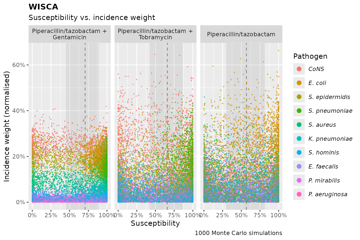
wisca_plot(wisca_out, wisca_plot_type = "posterior_coverage")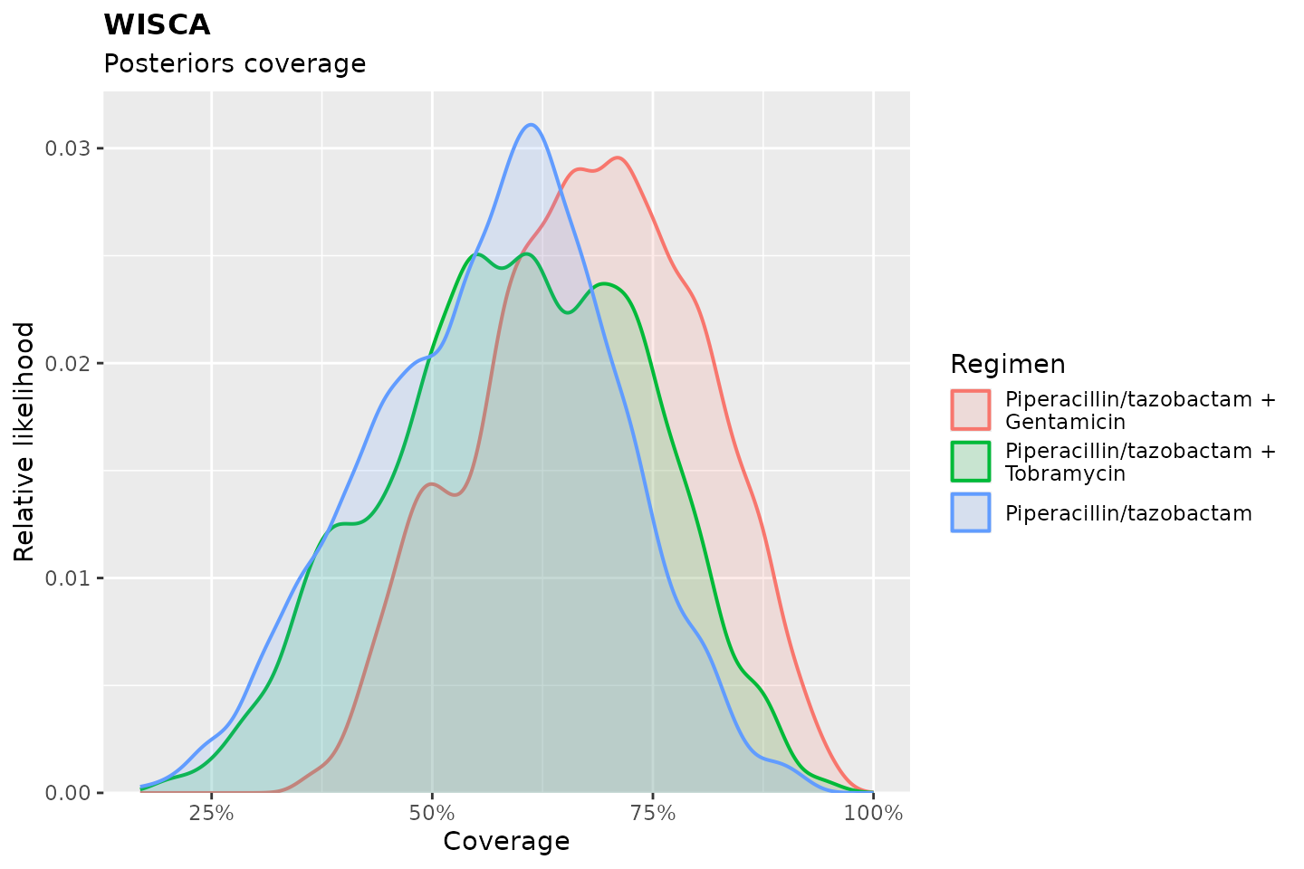
# a ggplot2 extension for WISCAs and other antibiograms:
ggplot2::autoplot(wisca_out)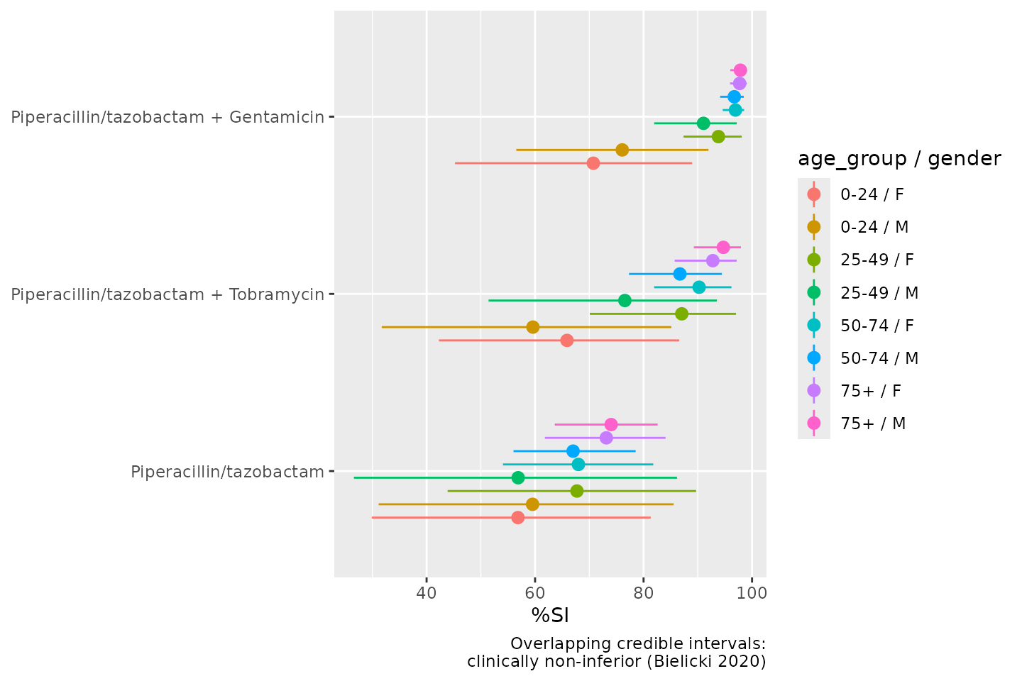
Traditional Antibiogram
If you need per-species susceptibility rates, e.g., for AMR surveillance reports, the traditional antibiogram remains the right tool. It reports the proportion of susceptible isolates per species per antibiotic:
antibiogram(example_isolates,
  antibiotics = c(aminoglycosides(), carbapenems())
)
#> ℹ For `aminoglycosides()` using columns GEN (gentamicin), TOB (tobramycin), AMK
#>   (amikacin), and KAN (kanamycin)
#> ℹ For `carbapenems()` using columns IPM (imipenem) and MEM (meropenem)| Pathogen | Amikacin | Gentamicin | Imipenem | Kanamycin | Meropenem | Tobramycin |
|---|---|---|---|---|---|---|
| CoNS | 0% (0-8%,N=43) | 86% (82-90%,N=309) | 52% (37-67%,N=48) | 0% (0-8%,N=43) | 52% (37-67%,N=48) | 22% (12-35%,N=55) |
| E. coli | 100% (98-100%,N=171) | 98% (96-99%,N=460) | 100% (99-100%,N=422) | NA | 100% (99-100%,N=418) | 97% (96-99%,N=462) |
| E. faecalis | 0% (0-9%,N=39) | 0% (0-9%,N=39) | 100% (91-100%,N=38) | 0% (0-9%,N=39) | NA | 0% (0-9%,N=39) |
| K. pneumoniae | NA | 90% (79-96%,N=58) | 100% (93-100%,N=51) | NA | 100% (93-100%,N=53) | 90% (79-96%,N=58) |
| P. aeruginosa | NA | 100% (88-100%,N=30) | NA | 0% (0-12%,N=30) | NA | 100% (88-100%,N=30) |
| P. mirabilis | NA | 94% (80-99%,N=34) | 94% (79-99%,N=32) | NA | NA | 94% (80-99%,N=34) |
| S. aureus | NA | 99% (97-100%,N=233) | NA | NA | NA | 98% (92-100%,N=86) |
| S. epidermidis | 0% (0-8%,N=44) | 79% (71-85%,N=163) | NA | 0% (0-8%,N=44) | NA | 51% (40-61%,N=89) |
| S. hominis | NA | 92% (84-97%,N=80) | NA | NA | NA | 85% (74-93%,N=62) |
| S. pneumoniae | 0% (0-3%,N=117) | 0% (0-3%,N=117) | NA | 0% (0-3%,N=117) | NA | 0% (0-3%,N=117) |
Notice that the antibiogram() function automatically
prints in the right format when using Quarto or R Markdown (such as this
page), and even applies italics for taxonomic names (by using
italicise_taxonomy() internally).
It also uses the language of your OS if this is either English,
Arabic, Bengali, Chinese, Czech, Danish, Dutch, Finnish, French, German,
Greek, Hindi, Indonesian, Italian, Japanese, Korean, Norwegian, Polish,
Portuguese, Romanian, Russian, Spanish, Swahili, Swedish, Turkish,
Ukrainian, Urdu, or Vietnamese. In this next example, we force the
language to be Spanish using the language argument:
antibiogram(example_isolates,
  mo_transform = "gramstain",
  antibiotics = aminoglycosides(),
  ab_transform = "name",
  language = "es"
)
#> ℹ For `aminoglycosides()` using columns GEN (gentamicin), TOB (tobramycin), AMK
#> (amikacin), and KAN (kanamycin)| Patógeno | Amikacina | Gentamicina | Kanamicina | Tobramicina |
|---|---|---|---|---|
| Gram negativo | 98% (96-99%,N=256) | 96% (95-98%,N=684) | 0% (0-10%,N=35) | 96% (94-97%,N=686) |
| Gram positivo | 0% (0-1%,N=436) | 63% (60-66%,N=1170) | 0% (0-1%,N=436) | 34% (31-38%,N=665) |
Combination Antibiogram
A combination antibiogram shows how much additional susceptibility a second agent adds for a given species. This is useful for surveillance of combination regimens, but note that it is still species-stratified and does not account for pathogen incidence in the syndrome:
combined_ab <- antibiogram(example_isolates,
  antibiotics = c("TZP", "TZP+TOB", "TZP+GEN"),
  ab_transform = NULL
)
combined_ab| Pathogen | TZP | TZP + GEN | TZP + TOB |
|---|---|---|---|
| CoNS | 30% (16-49%,N=33) | 97% (95-99%,N=274) | NA |
| E. coli | 94% (92-96%,N=416) | 100% (98-100%,N=459) | 99% (97-100%,N=461) |
| K. pneumoniae | 89% (77-96%,N=53) | 93% (83-98%,N=58) | 93% (83-98%,N=58) |
| P. aeruginosa | NA | 100% (88-100%,N=30) | 100% (88-100%,N=30) |
| P. mirabilis | NA | 100% (90-100%,N=34) | 100% (90-100%,N=34) |
| S. aureus | NA | 100% (98-100%,N=231) | 100% (96-100%,N=91) |
| S. epidermidis | NA | 100% (97-100%,N=128) | 100% (92-100%,N=46) |
| S. hominis | NA | 100% (95-100%,N=74) | 100% (93-100%,N=53) |
| S. pneumoniae | 100% (97-100%,N=112) | 100% (97-100%,N=112) | 100% (97-100%,N=112) |
Syndromic Antibiogram
A syndromic antibiogram stratifies per-species susceptibility by clinical context (ward, specimen type, etc.). It adds clinical context to the traditional antibiogram but is still species-level, without incidence weighting or uncertainty quantification. For surveillance by setting this is fine; for empirical therapy guidance, WISCA is preferred:
antibiogram(example_isolates,
  antibiotics = c(aminoglycosides(), carbapenems()),
  syndromic_group = "ward"
)
#> ℹ For `aminoglycosides()` using columns GEN (gentamicin), TOB (tobramycin), AMK
#>   (amikacin), and KAN (kanamycin)
#> ℹ For `carbapenems()` using columns IPM (imipenem) and MEM (meropenem)| Syndromic Group | Pathogen | Amikacin | Gentamicin | Imipenem | Kanamycin | Meropenem | Tobramycin |
|---|---|---|---|---|---|---|---|
| Clinical | CoNS | NA | 89% (84-93%,N=205) | 57% (39-74%,N=35) | NA | 57% (39-74%,N=35) | 26% (12-45%,N=31) |
| ICU | CoNS | NA | 79% (68-88%,N=73) | NA | NA | NA | NA |
| Outpatient | CoNS | NA | 84% (66-95%,N=31) | NA | NA | NA | NA |
| Clinical | E. coli | 100% (97-100%,N=104) | 98% (96-99%,N=297) | 100% (99-100%,N=266) | NA | 100% (99-100%,N=276) | 98% (96-99%,N=299) |
| ICU | E. coli | 100% (93-100%,N=52) | 99% (95-100%,N=137) | 100% (97-100%,N=133) | NA | 100% (97-100%,N=118) | 96% (92-99%,N=137) |
| Clinical | K. pneumoniae | NA | 92% (81-98%,N=51) | 100% (92-100%,N=44) | NA | 100% (92-100%,N=46) | 92% (81-98%,N=51) |
| Clinical | P. mirabilis | NA | 100% (88-100%,N=30) | NA | NA | NA | 100% (88-100%,N=30) |
| Clinical | S. aureus | NA | 99% (95-100%,N=150) | NA | NA | NA | 97% (89-100%,N=63) |
| ICU | S. aureus | NA | 100% (95-100%,N=66) | NA | NA | NA | NA |
| Clinical | S. epidermidis | NA | 82% (72-90%,N=79) | NA | NA | NA | 55% (39-70%,N=44) |
| ICU | S. epidermidis | NA | 72% (60-82%,N=75) | NA | NA | NA | 41% (26-58%,N=41) |
| Clinical | S. hominis | NA | 96% (85-99%,N=45) | NA | NA | NA | 94% (79-99%,N=31) |
| Clinical | S. pneumoniae | 0% (0-5%,N=78) | 0% (0-5%,N=78) | NA | 0% (0-5%,N=78) | NA | 0% (0-5%,N=78) |
| ICU | S. pneumoniae | 0% (0-12%,N=30) | 0% (0-12%,N=30) | NA | 0% (0-12%,N=30) | NA | 0% (0-12%,N=30) |
Plotting antibiograms
All antibiogram types, including WISCA, can be plotted using
autoplot() from the ggplot2 package, since
this AMR package provides an extension to that
function:
autoplot(wisca_result)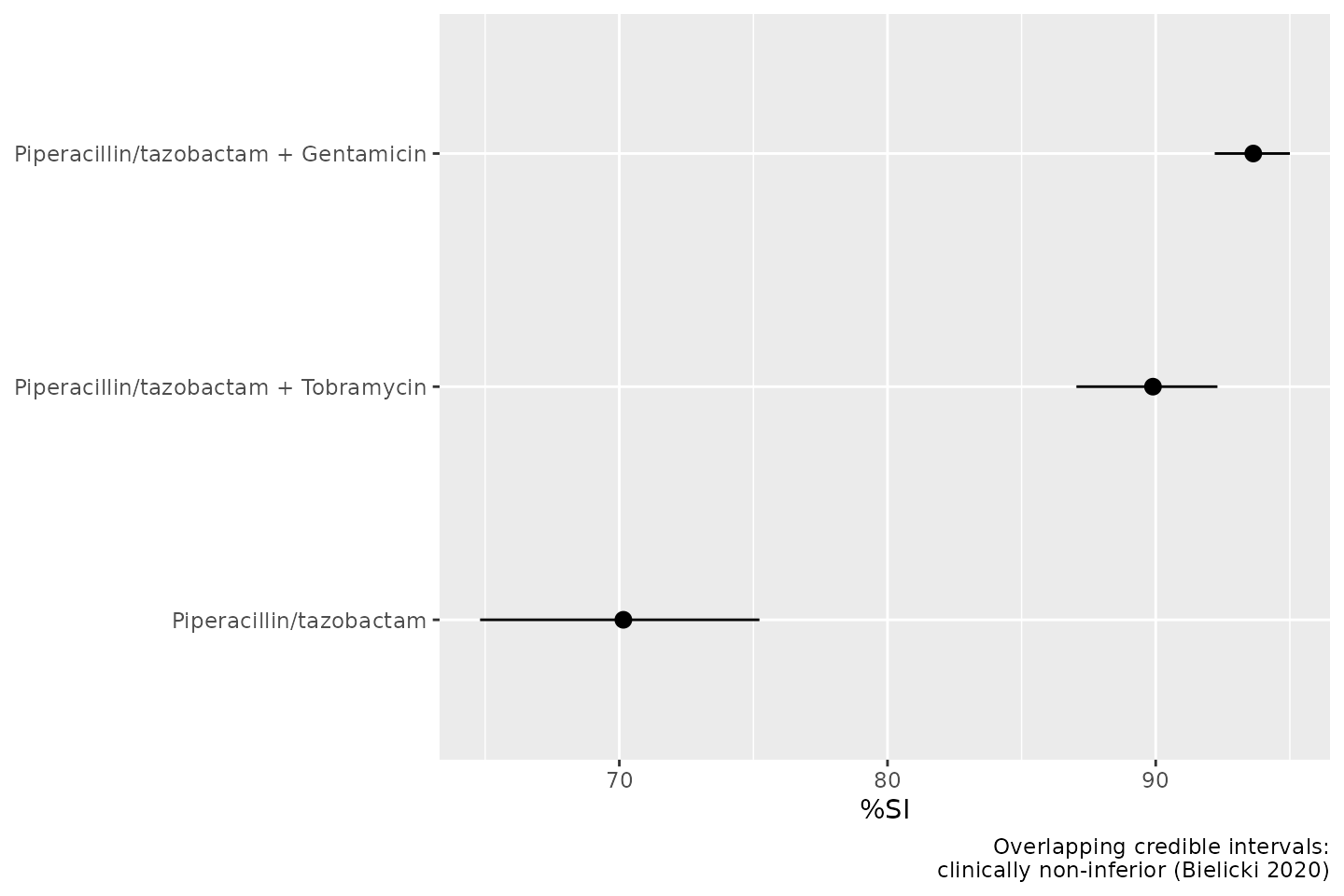
To calculate antimicrobial resistance in a more sensible way, also by
correcting for too few results, we use the resistance() and
susceptibility() functions.
Resistance percentages
The functions resistance() and
susceptibility() can be used to calculate antimicrobial
resistance or susceptibility. For more specific analyses, the functions
proportion_S(), proportion_SI(),
proportion_I(), proportion_IR() and
proportion_R() can be used to determine the proportion of a
specific antimicrobial outcome.
All these functions contain a minimum argument, denoting
the minimum required number of test results for returning a value. These
functions will otherwise return NA. The default is
minimum = 30, following the CLSI
M39-A4 guideline for applying microbial epidemiology.
As per the EUCAST guideline of 2019, we calculate resistance as the
proportion of R (proportion_R(), equal to
resistance()) and susceptibility as the proportion of S and
I (proportion_SI(), equal to
susceptibility()). These functions can be used on their
own:
our_data_1st %>% resistance(AMX)
#> ℹ `resistance()` assumes the EUCAST guideline and thus considers the 'I'
#>   category susceptible. Set the `guideline` argument or the `AMR_guideline`
#>   option to either "CLSI" or "EUCAST", see `?AMR-options`.
#> ℹ This message will be shown once per session.
#> [1] 0.4203377
Or can be used in conjunction with group_by() and
summarise(), both from the dplyr package:
our_data_1st %>%
  group_by(hospital) %>%
  summarise(amoxicillin = resistance(AMX))
#> # A tibble: 3 × 2
#>   hospital amoxicillin
#>   <chr>          <dbl>
#> 1 A              0.340
#> 2 B              0.551
#> 3 C              0.370
Interpreting MIC and Disk Diffusion Values
Minimal inhibitory concentration (MIC) values and disk diffusion
diameters can be interpreted into clinical breakpoints (SIR) using
as.sir(). Here’s an example with randomly generated MIC
values for Klebsiella pneumoniae and ciprofloxacin:
set.seed(123)
mic_values <- random_mic(100)
sir_values <- as.sir(mic_values, mo = "K. pneumoniae", ab = "cipro", guideline = "EUCAST 2024")

my_data <- tibble(MIC = mic_values, SIR = sir_values)
my_data
#> # A tibble: 100 × 2
#>         MIC SIR
#>       <mic> <sir>
#>  1 <=0.0001   S
#>  2   0.0160   S
#>  3 >=8.0000   R
#>  4   0.0320   S
#>  5   0.0080   S
#>  6  64.0000   R
#>  7   0.0080   S
#>  8   0.1250   S
#>  9   0.0320   S
#> 10   0.0002   S
#> # ℹ 90 more rows
This allows direct interpretation according to EUCAST or CLSI breakpoints, facilitating automated AMR data processing.
Plotting MIC and SIR Interpretations
We can visualise MIC distributions and their SIR interpretations
using ggplot2, using the new scale_y_mic() for
the y-axis and scale_colour_sir() to colour-code SIR
categories.
# add a group
my_data$group <- rep(c("A", "B", "C", "D"), each = 25)

ggplot(
  my_data,
  aes(x = group, y = MIC, colour = SIR)
) +
  geom_jitter(width = 0.2, size = 2) +
  geom_boxplot(fill = NA, colour = "grey40") +
  scale_y_mic() +
  scale_colour_sir() +
  labs(
    title = "MIC Distribution and SIR Interpretation",
    x = "Sample Groups",
    y = "MIC (mg/L)"
  )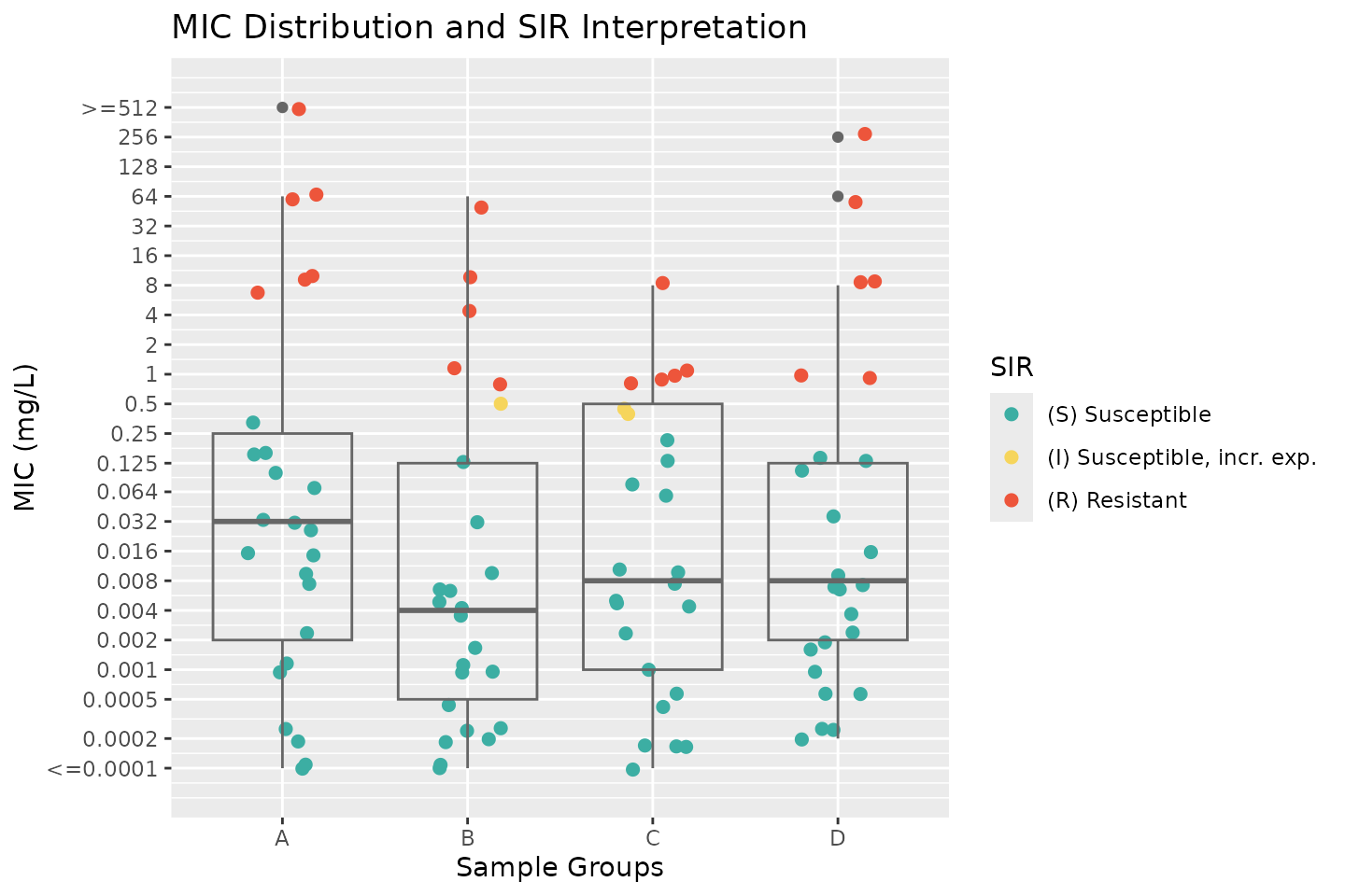
This plot provides an intuitive way to assess susceptibility patterns across different groups while incorporating clinical breakpoints.
For a more straightforward and less manual approach,
ggplot2’s function autoplot() has been
extended by this package to directly plot MIC and disk diffusion
values:
autoplot(mic_values)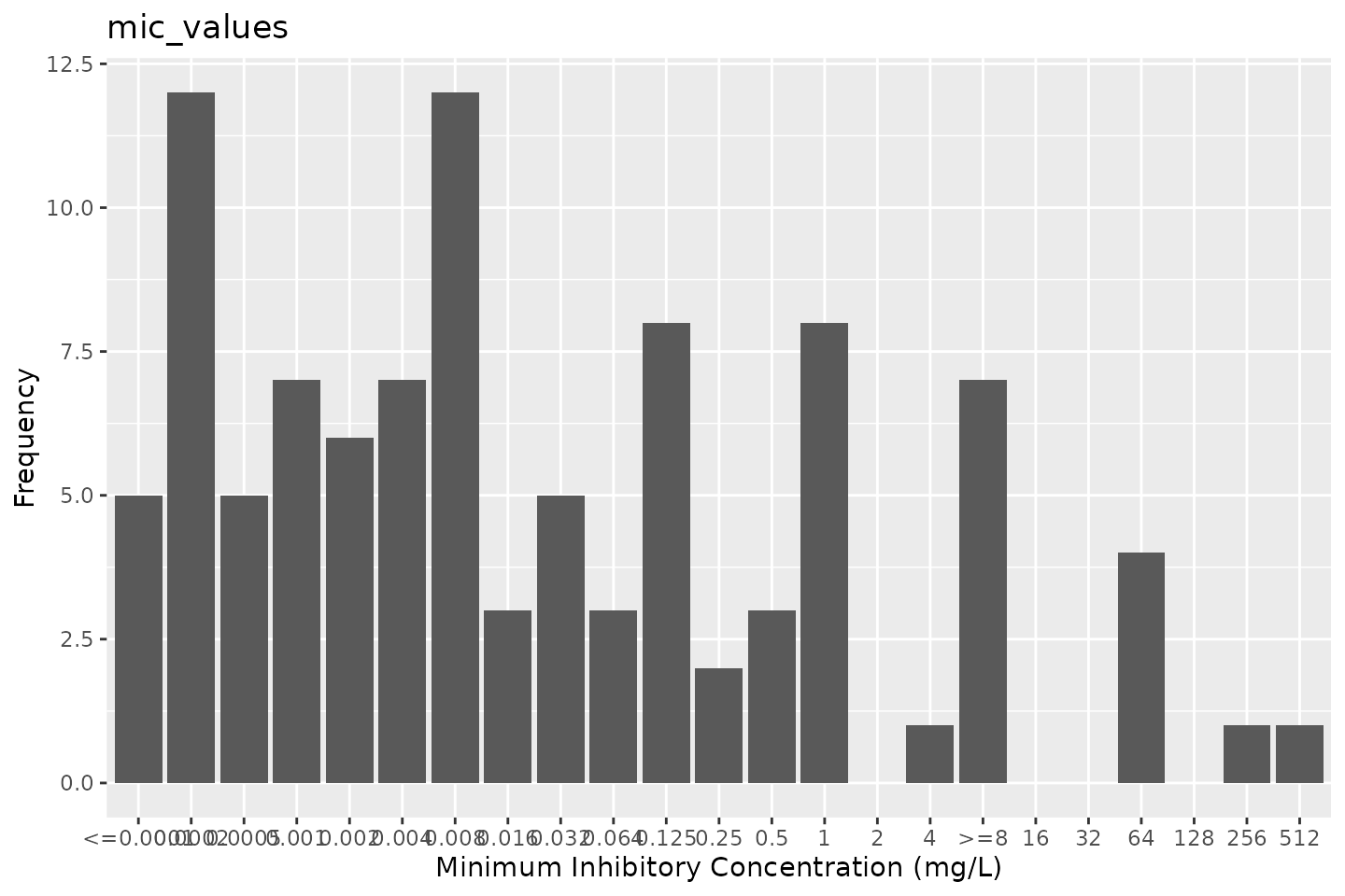
# by providing `mo` and `ab`, colours will indicate the SIR interpretation:
autoplot(mic_values, mo = "K. pneumoniae", ab = "cipro", guideline = "EUCAST 2024")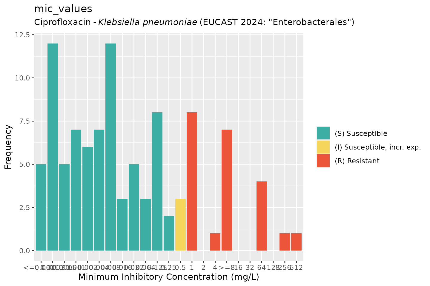
Author: Dr. Matthijs Berends, 23rd June 2026