Generate Antibiograms (WISCA, Traditional, Combination, or Syndromic)
Source:R/antibiogram.R
antibiogram.RdGenerate antibiograms from antimicrobial susceptibility data, with support for traditional, combination, syndromic, and WISCA (Weighted-Incidence Syndromic Combination Antibiogram) methods.
For empirical therapy guidance, WISCA is the recommended approach. When initiating empirical treatment, the causative pathogen is unknown, and the clinically relevant question is: "what is the probability that this regimen will cover whatever pathogen turns out to cause the infection?" WISCA answers that question directly by weighting susceptibility by pathogen incidence within a syndrome and providing credible intervals via Bayesian Monte Carlo simulation. Traditional antibiograms remain appropriate for tracking resistance per species for surveillance purposes. See the section Explaining WISCA on this page and the WISCA vignette for details.
All antibiogram types adhere to previously described approaches (see Source), and the WISCA method implements the Bayesian decision model by Bielicki et al. (2016, doi:10.1093/jac/dkv397 ). Output formats include plots and tables, ideal for integration with R Markdown and Quarto reports.
Usage
wisca(
  x,
  antimicrobials = where(is.sir),
  ab_transform = "name",
  syndromic_group = NULL,
  only_all_tested = FALSE,
  digits = 1,
  formatting_type = getOption("AMR_antibiogram_formatting_type", 14),
  col_mo = NULL,
  language = get_AMR_locale(),
  combine_SI = TRUE,
  sep = " + ",
  sort_columns = TRUE,
  simulations = 1000,
  conf_interval = 0.95,
  interval_side = "two-tailed",
  info = interactive(),
  parallel = FALSE,
  ...
)

antibiogram(
  x,
  antimicrobials = where(is.sir),
  mo_transform = "shortname",
  ab_transform = "name",
  syndromic_group = NULL,
  add_total_n = FALSE,
  only_all_tested = FALSE,
  digits = ifelse(wisca, 1, 0),
  formatting_type = getOption("AMR_antibiogram_formatting_type", ifelse(wisca, 14, 18)),
  col_mo = NULL,
  language = get_AMR_locale(),
  minimum = 30,
  combine_SI = TRUE,
  sep = " + ",
  sort_columns = TRUE,
  wisca = FALSE,
  simulations = 1000,
  conf_interval = 0.95,
  interval_side = "two-tailed",
  info = interactive(),
  parallel = FALSE,
  ...
)

retrieve_wisca_parameters(wisca_model, ...)

# S3 method for class 'antibiogram'
plot(x, ...)

# S3 method for class 'antibiogram'
autoplot(
  object,
  geom = c("pointrange", "point", "col", "bar", "errorbar"),
  ci = TRUE,
  sort = TRUE,
  flip = NULL,
  caption = NULL,
  ...
)

wisca_plot(
  wisca_model,
  wisca_plot_type = c("susceptibility_incidence", "posterior_coverage"),
  ...
)

# S3 method for class 'antibiogram'
knit_print(
  x,
  italicise = TRUE,
  na = getOption("knitr.kable.NA", default = ""),
  ...
)
Arguments
- x
A data.frame containing at least a column with microorganisms and columns with antimicrobial results (class 'sir', see
as.sir()).- antimicrobials
A vector specifying the antimicrobials containing SIR values to include in the antibiogram (see Examples). Will be evaluated using
guess_ab_col(). This can be:Any antimicrobial name or code that could match (see
guess_ab_col()) to any column inxAny antimicrobial selector, such as
aminoglycosides()orcarbapenems()A combination of the above, using
c(), e.g.:c(aminoglycosides(), "AMP", "AMC")c(aminoglycosides(), carbapenems())
Column indices using numbers
Combination therapy, indicated by using
"+", with or without antimicrobial selectors, e.g.:"cipro + genta""TZP+TOB"c("TZP", "TZP+GEN", "TZP+TOB")carbapenems() + "GEN"carbapenems() + c("", "GEN")carbapenems() + c("", aminoglycosides())
- ab_transform
A character to transform antimicrobial input - must be one of the column names of the antimicrobials data set (defaults to
"name"):"ab","cid","name","group","atc","atc_group1","atc_group2","abbreviations","synonyms","oral_ddd","oral_units","iv_ddd","iv_units", or"loinc". Can also beNULLto not transform the input.- syndromic_group
A column name of
x, or values calculated to split rows ofx, e.g. by usingifelse()orcase_when(). See Examples.- only_all_tested
(for combination antibiograms): a logical to indicate that isolates must be tested for all antimicrobials, see Details.
- digits
Number of digits to use for rounding the antimicrobial coverage, defaults to 1 for WISCA and 0 otherwise.
- formatting_type
Numeric value (1-22 for WISCA, 1-12 for non-WISCA) indicating how the 'cells' of the antibiogram table should be formatted. See Details > Formatting Type for a list of options.
- col_mo
Column name of the names or codes of the microorganisms (see
as.mo()) - the default is the first column of classmo. Values will be coerced usingas.mo().- language
Language to translate text, which defaults to the system language (see
get_AMR_locale()).- combine_SI
A logical to indicate whether all susceptibility should be determined by results of either S, SDD, or I, instead of only S (default is
TRUE).- sep
A separating character for antimicrobial columns in combination antibiograms.
- sort_columns
A logical to indicate whether the antimicrobial columns must be sorted on name.
- simulations
(for WISCA) a numerical value to set the number of Monte Carlo simulations.
- conf_interval
A numerical value to set confidence interval (default is
0.95).- interval_side
The side of the confidence interval, either
"two-tailed"(default),"left"or"right".- info
A logical to indicate info should be printed - the default is
TRUEonly in interactive mode.- parallel
A logical to indicate if parallel computing must be used, defaults to
FALSE. Requires thefuture.applypackage. For WISCA, Monte Carlo simulations are distributed across workers; for grouped antibiograms, each group is processed by a separate worker. A non-sequentialfuture::plan()must already be active before settingparallel = TRUE– for example,future::plan(future::multisession). An error is thrown ifparallel = TRUEis used without a plan set by the user.- ...
Currently unused.
- mo_transform
A character to transform microorganism input - must be
"name","shortname"(default),"gramstain", or one of the column names of the microorganisms data set:"mo","fullname","status","domain","kingdom","phylum","class","order","family","genus","species","subspecies","rank","ref","oxygen_tolerance","morphology","source","lpsn","lpsn_parent","lpsn_renamed_to","mycobank","mycobank_parent","mycobank_renamed_to","gbif","gbif_parent","gbif_renamed_to","prevalence", or"snomed". Can also beNULLto not transform the input orNAto consider all microorganisms 'unknown'.- add_total_n
(deprecated in favour of
formatting_type) A logical to indicate whethern_testedavailable numbers per pathogen should be added to the table (default isTRUE). This will add the lowest and highest number of available isolates per antimicrobial (e.g., if for E. coli 200 isolates are available for ciprofloxacin and 150 for amoxicillin, the returned number will be "150-200"). This option is unavailable whenwisca = TRUE; in that case, useretrieve_wisca_parameters()to get the parameters used for WISCA.- minimum
The minimum allowed number of available (tested) isolates. Any isolate count lower than
minimumwill returnNAwith a warning. The default number of30isolates is advised by the Clinical and Laboratory Standards Institute (CLSI) as best practice, see Source.- wisca
A logical to indicate whether a Weighted-Incidence Syndromic Combination Antibiogram (WISCA) must be generated (default is
FALSE). This will use a Bayesian decision model to estimate regimen coverage probabilities using Monte Carlo simulations. Per doi:10.1093/jac/dkv397 , susceptibility priors are \(\beta(0.5, 0.5)\) (Jeffreys) and intrinsically resistant pairs (based on intrinsic_resistant) use \(\beta(1, 9999)\).Set
simulations,conf_interval, andinterval_sideto adjust.- wisca_model
The outcome of
wisca()orantibiogram(..., wisca = TRUE).- object
An
antibiogram()object.- geom
The plotting style for the point estimate. One of
"pointrange"(default),"point","col"/"bar", or"errorbar"."pointrange"is recommended for coverage data: bars imply a meaningful baseline at zero, which coverage estimates rarely have.- ci
Logical, whether to draw the credible/confidence interval. Defaults to
TRUE. Ignored (forcedTRUE) whengeom = "pointrange"or"errorbar", since the interval is intrinsic to those geoms.- sort
Logical, whether to order regimens by coverage. Defaults to
TRUE. When faceted (per pathogen) or grouped (syndromic), ordering is applied within each panel/group.- flip
Logical, whether to draw regimens on the y-axis (horizontal). Defaults to
NULL, which flips automatically when any regimen label exceeds 20 characters (long combination names read poorly on the x-axis). SetTRUE/FALSEto override.- caption
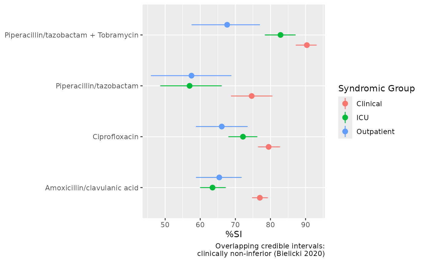
Text to show as caption, will explain non-inferiority for WISCA models.
- wisca_plot_type
Either
"susceptibility_incidence"(default) or"posterior_coverage".- italicise
A logical to indicate whether the microorganism names in the knitr table should be made italic, using
italicise_taxonomy().- na
Character to use for showing
NAvalues.
Details
These functions return a table with values between 0 and 100 for susceptibility, not resistance.
Remember that you should filter your data to let it contain only first isolates! This is needed to exclude duplicates and to reduce selection bias. Use first_isolate() to determine them with one of the four available algorithms: isolate-based, patient-based, episode-based, or phenotype-based.
For estimating antimicrobial coverage, especially when creating a WISCA, the outcome might become more reliable by only including the top n species encountered in the data. You can filter on this top n using top_n_microorganisms(). For example, use top_n_microorganisms(your_data, n = 10) as a pre-processing step to only include the top 10 species in the data.
The numeric values of an antibiogram are stored in a long format as the attribute long_numeric. You can retrieve them using attributes(x)$long_numeric, where x is the outcome of antibiogram() or wisca(). This is ideal for e.g. advanced plotting.
Formatting Type
The formatting of the 'cells' of the table can be set with the argument formatting_type. In these examples, 5 indicates the antimicrobial coverage (4-6 the confidence level), 15 the number of susceptible isolates, and 300 the number of tested (i.e., available) isolates:
5
15
300
15/300
5 (300)
5% (300)
5 (N=300)
5% (N=300)
5 (15/300)
5% (15/300)
5 (N=15/300)
5% (N=15/300)
5 (4-6)
5% (4-6%) - default for WISCA
5 (4-6,300)
5% (4-6%,300)
5 (4-6,N=300)
5% (4-6%,N=300) - default for non-WISCA
5 (4-6,15/300)
5% (4-6%,15/300)
5 (4-6,N=15/300)
5% (4-6%,N=15/300)
The default can be set globally with the package option AMR_antibiogram_formatting_type, e.g. options(AMR_antibiogram_formatting_type = 5). Do note that for WISCA, the total numbers of tested and susceptible isolates are less useful to report, since these are included in the Bayesian model and apparent from the susceptibility and its confidence level.
Set digits (defaults to 0) to alter the rounding of the susceptibility percentages.
When to Use WISCA vs. Traditional Antibiograms
There are various antibiogram types, as summarised by Klinker et al. (2021, doi:10.1177/20499361211011373
), and they are all supported by antibiogram(): traditional, combination, syndromic, and WISCA.
If your goal is to guide empirical therapy, use WISCA. Traditional antibiograms fragment susceptibility information by species, but at the point of prescribing, the clinician does not know which species is causing the infection. WISCA shifts the unit of analysis from the isolate to the patient: it estimates the probability that a regimen will cover the infection, given the local distribution of causative pathogens. It evaluates combination regimens, weights by pathogen incidence, and provides credible intervals that honestly communicate uncertainty. Hebert et al. (2012) demonstrated this concretely for the first time: ciprofloxacin showed 84% susceptibility against E. coli in the traditional antibiogram, but WISCA coverage was only 62% for UTI and 37% for abdominal infections, because other species (including intrinsically resistant enterococci) contribute substantially to these syndromes. Note that WISCA is pathogen-agnostic: the outcome is not stratified by species, but by syndrome.
Traditional, combination, and syndromic antibiograms remain appropriate for AMR surveillance, i.e., tracking resistance trends per species over time. They are the right tool when the question is "how resistant is species X to drug Y in our setting?" rather than "what regimen best covers this syndrome?".
All four types are demonstrated in the Examples section below.
Grouped tibbles
For any type of antibiogram, grouped tibbles can also be used to calculate susceptibilities over various groups.
Code example:
Inclusion in Combination Antibiograms
Note that for combination antibiograms, it is important to realise that susceptibility can be calculated in two ways, which can be set with the only_all_tested argument (default is FALSE). See this example for two antimicrobials, Drug A and Drug B, about how antibiogram() works to calculate the %SI:
--------------------------------------------------------------------
                    only_all_tested = FALSE  only_all_tested = TRUE
                    -----------------------  -----------------------
 Drug A    Drug B   considered   considered  considered   considered
                    susceptible    tested    susceptible    tested
--------  --------  -----------  ----------  -----------  ----------
 S or I    S or I        X            X           X            X
   R       S or I        X            X           X            X
  <NA>     S or I        X            X           -            -
 S or I      R           X            X           X            X
   R         R           -            X           -            X
  <NA>       R           -            -           -            -
 S or I     <NA>         X            X           -            -
   R        <NA>         -            -           -            -
  <NA>      <NA>         -            -           -            -
--------------------------------------------------------------------
Plotting
All types of antibiograms as listed above can be plotted (using ggplot2::autoplot() or base R's plot() and barplot()). As mentioned above, the numeric values of an antibiogram are stored in a long format as the attribute long_numeric. You can retrieve them using attributes(x)$long_numeric, where x is the outcome of antibiogram() or wisca().
The outcome of antibiogram() can also be used directly in R Markdown / Quarto (i.e., knitr) for reports. In this case, knitr::kable() will be applied automatically and microorganism names will even be printed in italics at default (see argument italicise).
You can also use functions from specific 'table reporting' packages to transform the output of antibiogram() to your needs, e.g. with flextable::as_flextable() or gt::gt().
Explaining WISCA
WISCA (Weighted-Incidence Syndromic Combination Antibiogram) estimates the probability that an empirical antimicrobial regimen will provide adequate coverage for a given infection syndrome, before the causative pathogen has been identified.
It does so by combining two quantities: the relative incidence of each pathogen within the syndrome (modelled as a Dirichlet distribution) and the susceptibility of each pathogen to the regimen (modelled as Beta distributions). These are combined via Monte Carlo simulation to produce a coverage estimate with a credible interval.
Prior distributions: Pathogen incidence uses a non-informative \(Dirichlet(1, 1, \ldots, 1)\) prior. Susceptibility proportions use the Jeffreys prior, \(\beta(0.5, 0.5)\), except for pathogen-drug combinations with known intrinsic resistance, which use a strongly informative \(\beta(1, 9999)\) prior that forces near-zero susceptibility regardless of observed data. Intrinsic resistance is determined using the intrinsic_resistant data set, which is based on 'EUCAST Expected Resistant Phenotypes' v1.2 (2023).
Interpreting the output: Overlapping credible intervals between regimens indicate no significant difference in coverage; if a narrower-spectrum regimen overlaps with a broader one, the narrower-spectrum option may be preferred on stewardship grounds. Non-overlapping intervals indicate a clinically meaningful difference. For small sample sizes, consider pooling data from multiple sites to improve precision, provided pathogen distributions are sufficiently similar (Bielicki et al., 2016).
For the full mathematical derivation and worked examples, see the WISCA vignette.
References
Hebert C et al. (2012). Demonstration of the weighted-incidence syndromic combination antibiogram: an empiric prescribing decision aid. Infection Control & Hospital Epidemiology 33(4):381-388; doi:10.1086/664768
Bielicki JA et al. (2016). Selecting appropriate empirical antibiotic regimens for paediatric bloodstream infections: application of a Bayesian decision model to local and pooled antimicrobial resistance surveillance data. Journal of Antimicrobial Chemotherapy 71(3):794-802; doi:10.1093/jac/dkv397
Cook A et al. (2022). Improving empiric antibiotic prescribing in pediatric bloodstream infections: a potential application of weighted-incidence syndromic combination antibiograms (WISCA). Expert Review of Anti-infective Therapy 20(3):445-456; doi:10.1080/14787210.2021.1967145
Klinker KP et al. (2021). Antimicrobial stewardship and antibiograms: importance of moving beyond traditional antibiograms. Therapeutic Advances in Infectious Disease, May 5;8:20499361211011373; doi:10.1177/20499361211011373
Barbieri E et al. (2021). Development of a Weighted-Incidence Syndromic Combination Antibiogram (WISCA) to guide the choice of the empiric antibiotic treatment for urinary tract infection in paediatric patients: a Bayesian approach. Antimicrobial Resistance & Infection Control May 1;10(1):74; doi:10.1186/s13756-021-00939-2
M39 Analysis and Presentation of Cumulative Antimicrobial Susceptibility Test Data, 5th Edition, 2022, Clinical and Laboratory Standards Institute (CLSI). https://clsi.org/standards/products/microbiology/documents/m39/.
Examples
# example_isolates is a data set available in the AMR package.
# run ?example_isolates for more info.
example_isolates
#> # A tibble: 2,000 × 46
#> date patient age gender ward mo PEN OXA FLC AMX
#> <date> <chr> <dbl> <chr> <chr> <mo> <sir> <sir> <sir> <sir>
#> 1 2002-01-02 A77334 65 F Clinical B_ESCHR_COLI R NA NA NA
#> 2 2002-01-03 A77334 65 F Clinical B_ESCHR_COLI R NA NA NA
#> 3 2002-01-07 067927 45 F ICU B_STPHY_EPDR R NA R NA
#> 4 2002-01-07 067927 45 F ICU B_STPHY_EPDR R NA R NA
#> 5 2002-01-13 067927 45 F ICU B_STPHY_EPDR R NA R NA
#> 6 2002-01-13 067927 45 F ICU B_STPHY_EPDR R NA R NA
#> 7 2002-01-14 462729 78 M Clinical B_STPHY_AURS R NA S R
#> 8 2002-01-14 462729 78 M Clinical B_STPHY_AURS R NA S R
#> 9 2002-01-16 067927 45 F ICU B_STPHY_EPDR R NA R NA
#> 10 2002-01-17 858515 79 F ICU B_STPHY_EPDR R NA S NA
#> # ℹ 1,990 more rows
#> # ℹ 36 more variables: AMC <sir>, AMP <sir>, TZP <sir>, CZO <sir>, FEP <sir>,
#> # CXM <sir>, FOX <sir>, CTX <sir>, CAZ <sir>, CRO <sir>, GEN <sir>,
#> # TOB <sir>, AMK <sir>, KAN <sir>, TMP <sir>, SXT <sir>, NIT <sir>,
#> # FOS <sir>, LNZ <sir>, CIP <sir>, MFX <sir>, VAN <sir>, TEC <sir>,
#> # TCY <sir>, TGC <sir>, DOX <sir>, ERY <sir>, CLI <sir>, AZM <sir>,
#> # IPM <sir>, MEM <sir>, MTR <sir>, CHL <sir>, COL <sir>, MUP <sir>, …
# \donttest{
# WISCA antibiogram (recommended for empirical therapy) -----------------
# basic WISCA: empirical coverage per regimen, weighted by pathogen
# incidence, with 95% credible intervals
wisca(example_isolates,
antimicrobials = c("AMC", "AMC+CIP", "AMC+GEN")
)
#> Warning: invalid microorganism code, NA generated
#> # A tibble: 1 × 3
#> # Type: Weighted-Incidence Syndromic Combination Antibiogram (WISCA)
#> # Cred. interval: 95%
#> # Simulations: 1000 per stratum
#> `Amoxicillin/clavulanic acid` Amoxicillin/clavulanic …¹ Amoxicillin/clavulan…²
#> <chr> <chr> <chr>
#> 1 74.2% (72.1-76.1%) 88.8% (87.2-90.3%) 90.8% (89.3-92.1%)
#> # ℹ abbreviated names: ¹`Amoxicillin/clavulanic acid + Ciprofloxacin`,
#> # ²`Amoxicillin/clavulanic acid + Gentamicin`
#> # Use `ggplot2::autoplot()` or base R `plot()` to create a plot of this antibiogram,
#> # and use `wisca_plot()` to assess the simulation outcomes.
#> # Or, use it directly in R Markdown or Quarto, see `antibiogram()`.
# equivalent using antibiogram():
antibiogram(example_isolates,
antimicrobials = c("AMC", "AMC+CIP", "AMC+GEN"),
wisca = TRUE
)
#> Warning: invalid microorganism code, NA generated
#> # A tibble: 1 × 3
#> # Type: Weighted-Incidence Syndromic Combination Antibiogram (WISCA)
#> # Cred. interval: 95%
#> # Simulations: 1000 per stratum
#> `Amoxicillin/clavulanic acid` Amoxicillin/clavulanic …¹ Amoxicillin/clavulan…²
#> <chr> <chr> <chr>
#> 1 74.2% (72.2-76.1%) 88.8% (87.1-90.4%) 90.8% (89.4-92.2%)
#> # ℹ abbreviated names: ¹`Amoxicillin/clavulanic acid + Ciprofloxacin`,
#> # ²`Amoxicillin/clavulanic acid + Gentamicin`
#> # Use `ggplot2::autoplot()` or base R `plot()` to create a plot of this antibiogram,
#> # and use `wisca_plot()` to assess the simulation outcomes.
#> # Or, use it directly in R Markdown or Quarto, see `antibiogram()`.
# stratified by syndrome or clinical group
out <- wisca(example_isolates,
antimicrobials = c("TZP", "TZP+TOB", "TZP+GEN"),
syndromic_group = "ward"
)
#> Warning: invalid microorganism code, NA generated
out
#> # A tibble: 3 × 4
#> # Type: Weighted-Incidence Syndromic Combination Antibiogram (WISCA)
#> # Cred. interval: 95%
#> # Simulations: 1000 per stratum
#> `Syndromic Group` `Piperacillin/tazobactam` Piperacillin/tazobactam + Gentam…¹
#> <chr> <chr> <chr>
#> 1 Clinical 74.5% (68.8-79.8%) 93.6% (91.9-95.1%)
#> 2 ICU 57.1% (48.2-65.9%) 86.7% (83.3-89.9%)
#> 3 Outpatient 57.5% (46-68.7%) 76.5% (70.6-82.2%)
#> # ℹ abbreviated name: ¹`Piperacillin/tazobactam + Gentamicin`
#> # ℹ 1 more variable: `Piperacillin/tazobactam + Tobramycin` <chr>
#> # Use `ggplot2::autoplot()` or base R `plot()` to create a plot of this antibiogram,
#> # and use `wisca_plot()` to assess the simulation outcomes.
#> # Or, use it directly in R Markdown or Quarto, see `antibiogram()`.
wisca_plot(out)
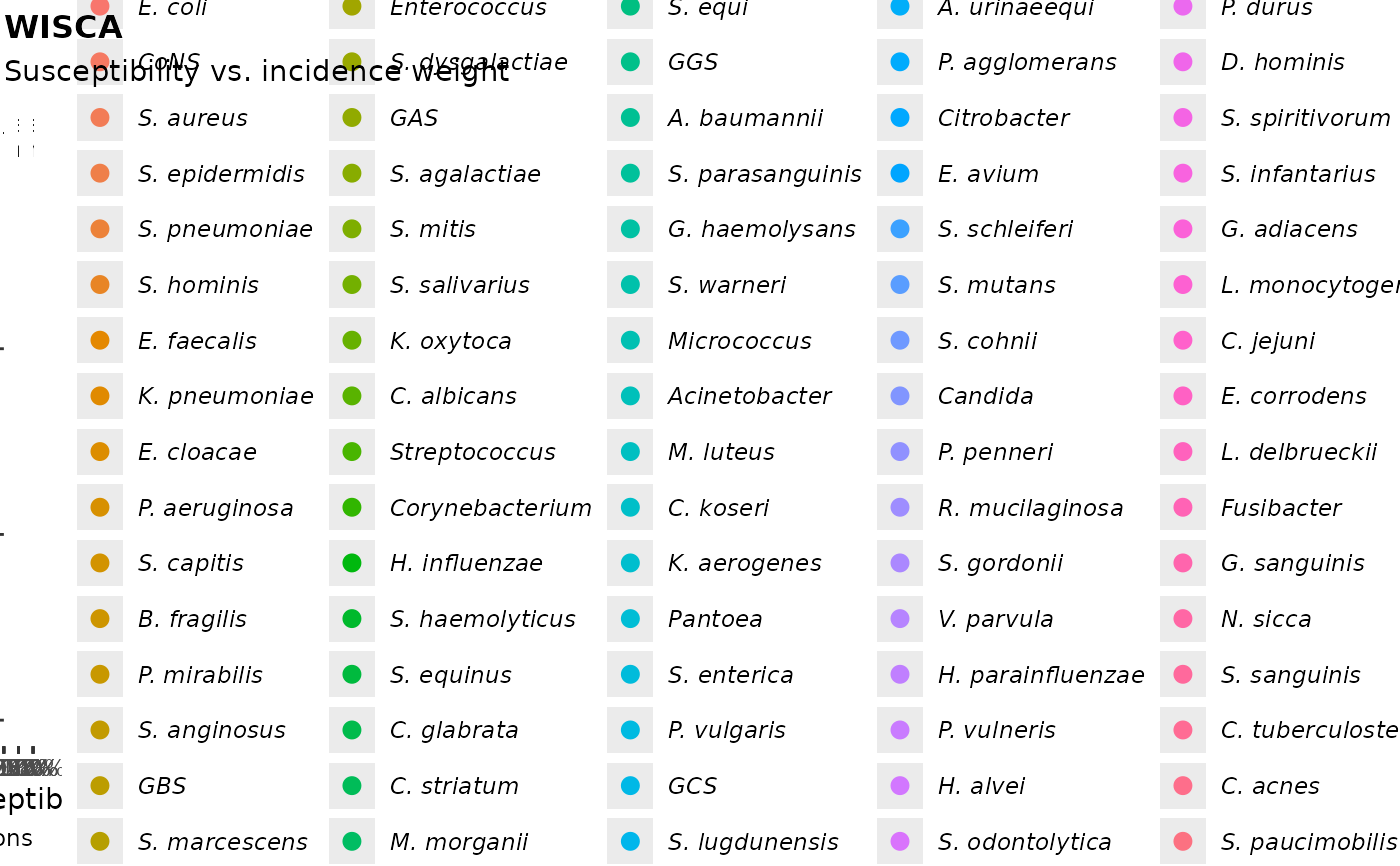 # stratified using grouped tibbles (e.g. by age and gender)
if (requireNamespace("dplyr")) {
library(dplyr)
example_isolates %>%
top_n_microorganisms(n = 10) %>%
group_by(
age_group = age_groups(age, c(25, 50, 75)),
gender) %>%
wisca(antimicrobials = c("TZP", "TZP+TOB", "TZP+GEN"))
}
#> ℹ Using column mo as input for `col_mo`.
#> Warning: Number of tested isolates should exceed 30 for each regimen (and group). WISCA
#> coverage estimates might be inaccurate.
#> # A tibble: 8 × 5
#> # Type: Weighted-Incidence Syndromic Combination Antibiogram (WISCA)
#> # Cred. interval: 95%
#> # Simulations: 1000 per stratum
#> age_group gender `Piperacillin/tazobactam` Piperacillin/tazobactam + Gentami…¹
#> <chr> <chr> <chr> <chr>
#> 1 0-24 F 57.7% (29.5-82.6%) 70.5% (45.9-89.1%)
#> 2 0-24 M 59.1% (33-84.2%) 76.1% (55.7-90.6%)
#> 3 25-49 F 67.4% (43.3-90.5%) 93.8% (87.8-97.9%)
#> 4 25-49 M 56.8% (27.5-86.5%) 90.9% (82.4-96.8%)
#> 5 50-74 F 68% (53.3-82.3%) 96.9% (94.7-98.5%)
#> 6 50-74 M 67.1% (56.5-77.5%) 96.8% (94.2-98.8%)
#> 7 75+ F 73.3% (62.9-83.6%) 97.7% (96-98.9%)
#> 8 75+ M 74% (64.2-83.1%) 97.9% (96.1-99.1%)
#> # ℹ abbreviated name: ¹`Piperacillin/tazobactam + Gentamicin`
#> # ℹ 1 more variable: `Piperacillin/tazobactam + Tobramycin` <chr>
#> # Use `ggplot2::autoplot()` or base R `plot()` to create a plot of this antibiogram,
#> # and use `wisca_plot()` to assess the simulation outcomes.
#> # Or, use it directly in R Markdown or Quarto, see `antibiogram()`.
# Traditional antibiogram (for AMR surveillance) ------------------------
antibiogram(example_isolates,
antimicrobials = c(aminoglycosides(), carbapenems())
)
#> ℹ For `aminoglycosides()` using columns GEN (gentamicin), TOB (tobramycin), AMK
#> (amikacin), and KAN (kanamycin)
#> ℹ For `carbapenems()` using columns IPM (imipenem) and MEM (meropenem)
#> # A tibble: 10 × 7
#> # Type: Traditional Antibiogram
#> # Conf. interval: 95%
#> Pathogen Amikacin Gentamicin Imipenem Kanamycin Meropenem Tobramycin
#> <chr> <chr> <chr> <chr> <chr> <chr> <chr>
#> 1 CoNS 0% (0-8%,N… 86% (82-9… 52% (37… 0% (0-8%… 52% (37-… 22% (12-3…
#> 2 E. coli 100% (98-1… 98% (96-9… 100% (9… NA 100% (99… 97% (96-9…
#> 3 E. faecalis 0% (0-9%,N… 0% (0-9%,… 100% (9… 0% (0-9%… NA 0% (0-9%,…
#> 4 K. pneumoniae NA 90% (79-9… 100% (9… NA 100% (93… 90% (79-9…
#> 5 P. aeruginosa NA 100% (88-… NA 0% (0-12… NA 100% (88-…
#> 6 P. mirabilis NA 94% (80-9… 94% (79… NA NA 94% (80-9…
#> 7 S. aureus NA 99% (97-1… NA NA NA 98% (92-1…
#> 8 S. epidermidis 0% (0-8%,N… 79% (71-8… NA 0% (0-8%… NA 51% (40-6…
#> 9 S. hominis NA 92% (84-9… NA NA NA 85% (74-9…
#> 10 S. pneumoniae 0% (0-3%,N… 0% (0-3%,… NA 0% (0-3%… NA 0% (0-3%,…
#> # Use `ggplot2::autoplot()` or base R `plot()` to create a plot of this antibiogram,
#> # or use it directly in R Markdown or Quarto, see `antibiogram()`.
antibiogram(example_isolates,
antimicrobials = aminoglycosides(),
ab_transform = "atc",
mo_transform = "gramstain"
)
#> ℹ For `aminoglycosides()` using columns GEN (gentamicin), TOB (tobramycin), AMK
#> (amikacin), and KAN (kanamycin)
#> # A tibble: 2 × 5
#> # Type: Traditional Antibiogram
#> # Conf. interval: 95%
#> Pathogen J01GB01 J01GB03 J01GB04 J01GB06
#> <chr> <chr> <chr> <chr> <chr>
#> 1 Gram-negative 96% (94-97%,N=686) 96% (95-98%,N=684) 0% (0-10%,N=35) 98% (96-…
#> 2 Gram-positive 34% (31-38%,N=665) 63% (60-66%,N=1170) 0% (0-1%,N=436) 0% (0-1%…
#> # Use `ggplot2::autoplot()` or base R `plot()` to create a plot of this antibiogram,
#> # or use it directly in R Markdown or Quarto, see `antibiogram()`.
# Combination antibiogram (for AMR surveillance) ------------------------
antibiogram(example_isolates,
antimicrobials = c("TZP", "TZP+TOB", "TZP+GEN"),
mo_transform = "gramstain"
)
#> # A tibble: 2 × 4
#> # Type: Combination Antibiogram
#> # Conf. interval: 95%
#> Pathogen Piperacillin/tazobac…¹ Piperacillin/tazobac…² Piperacillin/tazobac…³
#> <chr> <chr> <chr> <chr>
#> 1 Gram-neg… 88% (85-91%,N=641) 99% (97-99%,N=691) 98% (97-99%,N=693)
#> 2 Gram-pos… 86% (82-89%,N=345) 98% (96-98%,N=1044) 95% (93-97%,N=550)
#> # ℹ abbreviated names: ¹`Piperacillin/tazobactam`,
#> # ²`Piperacillin/tazobactam + Gentamicin`,
#> # ³`Piperacillin/tazobactam + Tobramycin`
#> # Use `ggplot2::autoplot()` or base R `plot()` to create a plot of this antibiogram,
#> # or use it directly in R Markdown or Quarto, see `antibiogram()`.
# you can use any antimicrobial selector with `+` too:
antibiogram(example_isolates,
antimicrobials = ureidopenicillins() + c("", "GEN", "tobra"),
mo_transform = "gramstain"
)
#> ℹ For `ureidopenicillins()` using column TZP (piperacillin/tazobactam)
#> # A tibble: 2 × 4
#> # Type: Combination Antibiogram
#> # Conf. interval: 95%
#> Pathogen Piperacillin/tazobac…¹ Piperacillin/tazobac…² Piperacillin/tazobac…³
#> <chr> <chr> <chr> <chr>
#> 1 Gram-neg… 88% (85-91%,N=641) 99% (97-99%,N=691) 98% (97-99%,N=693)
#> 2 Gram-pos… 86% (82-89%,N=345) 98% (96-98%,N=1044) 95% (93-97%,N=550)
#> # ℹ abbreviated names: ¹`Piperacillin/tazobactam`,
#> # ²`Piperacillin/tazobactam + Gentamicin`,
#> # ³`Piperacillin/tazobactam + Tobramycin`
#> # Use `ggplot2::autoplot()` or base R `plot()` to create a plot of this antibiogram,
#> # or use it directly in R Markdown or Quarto, see `antibiogram()`.
# names of antimicrobials do not need to resemble columns exactly:
antibiogram(example_isolates,
antimicrobials = c("Cipro", "cipro + genta"),
mo_transform = "gramstain",
ab_transform = "name",
sep = " & "
)
#> # A tibble: 2 × 3
#> # Type: Traditional Antibiogram
#> # Conf. interval: 95%
#> Pathogen Ciprofloxacin `Ciprofloxacin & Gentamicin`
#> <chr> <chr> <chr>
#> 1 Gram-negative 91% (88-93%,N=684) 99% (97-99%,N=694)
#> 2 Gram-positive 77% (74-80%,N=724) 93% (91-94%,N=847)
#> # Use `ggplot2::autoplot()` or base R `plot()` to create a plot of this antibiogram,
#> # or use it directly in R Markdown or Quarto, see `antibiogram()`.
# Syndromic antibiogram (for AMR surveillance) --------------------------
antibiogram(example_isolates,
antimicrobials = c(aminoglycosides(), carbapenems()),
syndromic_group = "ward"
)
#> ℹ For `aminoglycosides()` using columns GEN (gentamicin), TOB (tobramycin), AMK
#> (amikacin), and KAN (kanamycin)
#> ℹ For `carbapenems()` using columns IPM (imipenem) and MEM (meropenem)
#> # A tibble: 14 × 8
#> # Type: Syndromic Antibiogram
#> # Conf. interval: 95%
#> `Syndromic Group` Pathogen Amikacin Gentamicin Imipenem Kanamycin Meropenem
#> <chr> <chr> <chr> <chr> <chr> <chr> <chr>
#> 1 Clinical CoNS NA 89% (84-9… 57% (39… NA 57% (39-…
#> 2 ICU CoNS NA 79% (68-8… NA NA NA
#> 3 Outpatient CoNS NA 84% (66-9… NA NA NA
#> 4 Clinical E. coli 100% (9… 98% (96-9… 100% (9… NA 100% (99…
#> 5 ICU E. coli 100% (9… 99% (95-1… 100% (9… NA 100% (97…
#> 6 Clinical K. pneumo… NA 92% (81-9… 100% (9… NA 100% (92…
#> 7 Clinical P. mirabi… NA 100% (88-… NA NA NA
#> 8 Clinical S. aureus NA 99% (95-1… NA NA NA
#> 9 ICU S. aureus NA 100% (95-… NA NA NA
#> 10 Clinical S. epider… NA 82% (72-9… NA NA NA
#> 11 ICU S. epider… NA 72% (60-8… NA NA NA
#> 12 Clinical S. hominis NA 96% (85-9… NA NA NA
#> 13 Clinical S. pneumo… 0% (0-5… 0% (0-5%,… NA 0% (0-5%… NA
#> 14 ICU S. pneumo… 0% (0-1… 0% (0-12%… NA 0% (0-12… NA
#> # ℹ 1 more variable: Tobramycin <chr>
#> # Use `ggplot2::autoplot()` or base R `plot()` to create a plot of this antibiogram,
#> # or use it directly in R Markdown or Quarto, see `antibiogram()`.
# with a custom language, though this will be determined automatically
# (i.e., this table will be in Spanish on Spanish systems)
ex1 <- example_isolates[which(mo_genus() == "Escherichia"), ]
#> ℹ Using column mo as input for `mo_genus()`
antibiogram(ex1,
antimicrobials = aminoglycosides(),
ab_transform = "name",
syndromic_group = ifelse(ex1$ward == "ICU",
"UCI", "No UCI"
),
language = "es"
)
#> ℹ For `aminoglycosides()` using columns GEN (gentamicin), TOB (tobramycin), AMK
#> (amikacin), and KAN (kanamycin)
#> # A tibble: 2 × 5
#> # Type: Syndromic Antibiogram
#> # Conf. interval: 95%
#> `Grupo sindrómico` Patógeno Amikacina Gentamicina Tobramicina
#> <chr> <chr> <chr> <chr> <chr>
#> 1 No UCI E. coli 100% (97-100%,N=119) 98% (96-99%,N=32… 98% (96-99…
#> 2 UCI E. coli 100% (93-100%,N=52) 99% (95-100%,N=1… 96% (92-99…
#> # Use `ggplot2::autoplot()` or base R `plot()` to create a plot of this antibiogram,
#> # or use it directly in R Markdown or Quarto, see `antibiogram()`.
# Print the output for R Markdown / Quarto -----------------------------
ureido <- wisca(example_isolates,
antimicrobials = ureidopenicillins(),
syndromic_group = "ward"
)
#> ℹ For `ureidopenicillins()` using column TZP (piperacillin/tazobactam)
#> Warning: invalid microorganism code, NA generated
# in an Rmd file, you would just need to return `ureido` in a chunk,
# but to be explicit here:
if (requireNamespace("knitr")) {
cat(knitr::knit_print(ureido))
}
#>
#>
#> |Syndromic Group |Piperacillin/tazobactam |
#> |:---------------|:-----------------------|
#> |Clinical |74.6% (68.9-80%) |
#> |ICU |57% (49.1-65.8%) |
#> |Outpatient |57.4% (45.6-68.4%) |
# Generate plots with ggplot2 or base R --------------------------------
ab1 <- antibiogram(example_isolates,
antimicrobials = c("AMC", "CIP", "TZP", "TZP+TOB"),
mo_transform = "gramstain"
)
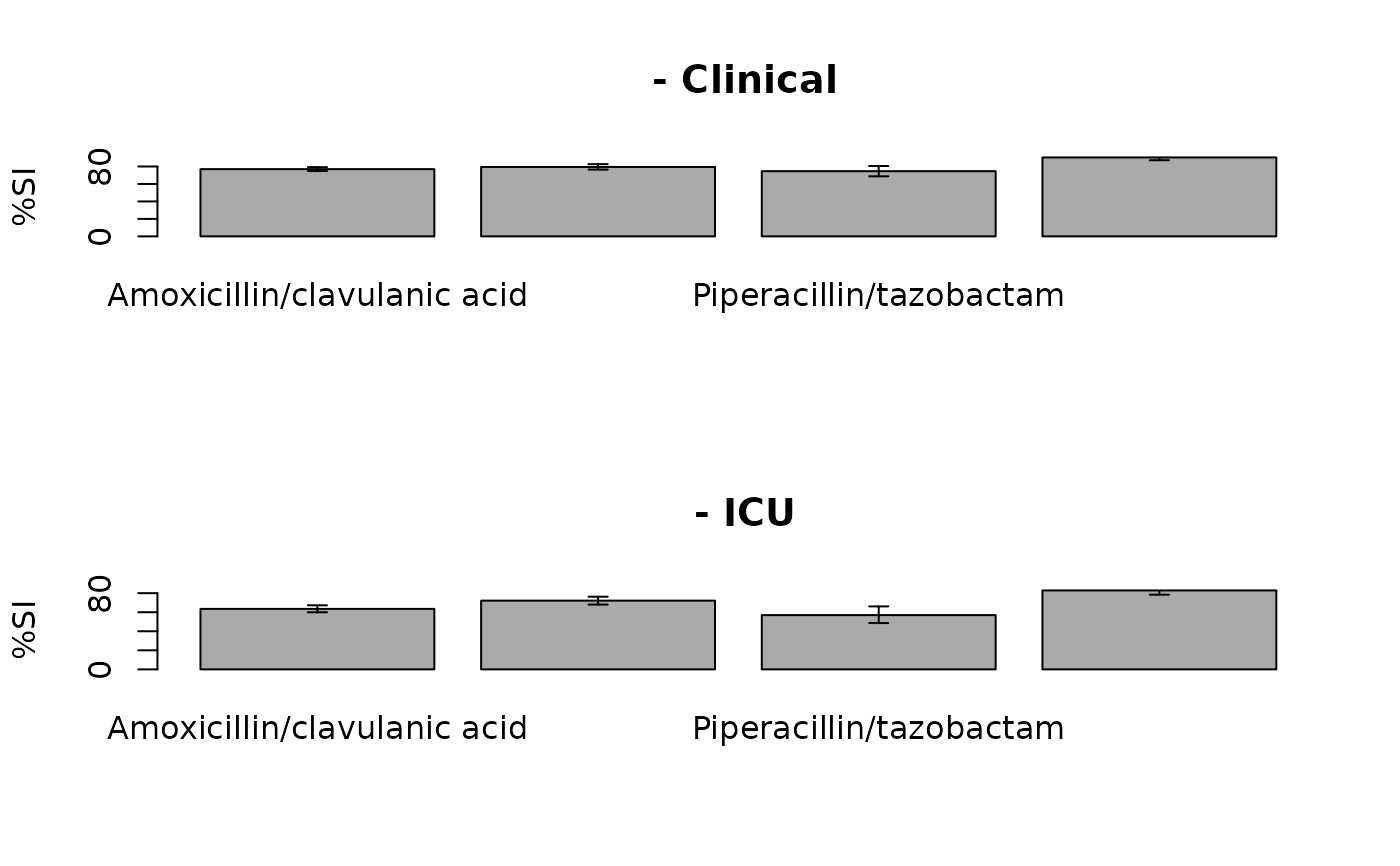
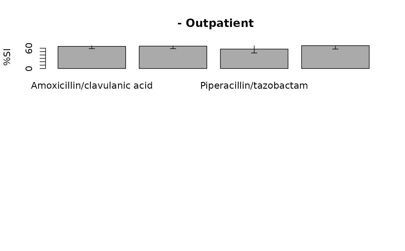
ab2 <- wisca(example_isolates,
antimicrobials = c("AMC", "CIP", "TZP", "TZP+TOB"),
syndromic_group = "ward"
)
#> Warning: invalid microorganism code, NA generated
if (requireNamespace("ggplot2")) {
ggplot2::autoplot(ab1)
}
# stratified using grouped tibbles (e.g. by age and gender)
if (requireNamespace("dplyr")) {
library(dplyr)
example_isolates %>%
top_n_microorganisms(n = 10) %>%
group_by(
age_group = age_groups(age, c(25, 50, 75)),
gender) %>%
wisca(antimicrobials = c("TZP", "TZP+TOB", "TZP+GEN"))
}
#> ℹ Using column mo as input for `col_mo`.
#> Warning: Number of tested isolates should exceed 30 for each regimen (and group). WISCA
#> coverage estimates might be inaccurate.
#> # A tibble: 8 × 5
#> # Type: Weighted-Incidence Syndromic Combination Antibiogram (WISCA)
#> # Cred. interval: 95%
#> # Simulations: 1000 per stratum
#> age_group gender `Piperacillin/tazobactam` Piperacillin/tazobactam + Gentami…¹
#> <chr> <chr> <chr> <chr>
#> 1 0-24 F 57.7% (29.5-82.6%) 70.5% (45.9-89.1%)
#> 2 0-24 M 59.1% (33-84.2%) 76.1% (55.7-90.6%)
#> 3 25-49 F 67.4% (43.3-90.5%) 93.8% (87.8-97.9%)
#> 4 25-49 M 56.8% (27.5-86.5%) 90.9% (82.4-96.8%)
#> 5 50-74 F 68% (53.3-82.3%) 96.9% (94.7-98.5%)
#> 6 50-74 M 67.1% (56.5-77.5%) 96.8% (94.2-98.8%)
#> 7 75+ F 73.3% (62.9-83.6%) 97.7% (96-98.9%)
#> 8 75+ M 74% (64.2-83.1%) 97.9% (96.1-99.1%)
#> # ℹ abbreviated name: ¹`Piperacillin/tazobactam + Gentamicin`
#> # ℹ 1 more variable: `Piperacillin/tazobactam + Tobramycin` <chr>
#> # Use `ggplot2::autoplot()` or base R `plot()` to create a plot of this antibiogram,
#> # and use `wisca_plot()` to assess the simulation outcomes.
#> # Or, use it directly in R Markdown or Quarto, see `antibiogram()`.
# Traditional antibiogram (for AMR surveillance) ------------------------
antibiogram(example_isolates,
antimicrobials = c(aminoglycosides(), carbapenems())
)
#> ℹ For `aminoglycosides()` using columns GEN (gentamicin), TOB (tobramycin), AMK
#> (amikacin), and KAN (kanamycin)
#> ℹ For `carbapenems()` using columns IPM (imipenem) and MEM (meropenem)
#> # A tibble: 10 × 7
#> # Type: Traditional Antibiogram
#> # Conf. interval: 95%
#> Pathogen Amikacin Gentamicin Imipenem Kanamycin Meropenem Tobramycin
#> <chr> <chr> <chr> <chr> <chr> <chr> <chr>
#> 1 CoNS 0% (0-8%,N… 86% (82-9… 52% (37… 0% (0-8%… 52% (37-… 22% (12-3…
#> 2 E. coli 100% (98-1… 98% (96-9… 100% (9… NA 100% (99… 97% (96-9…
#> 3 E. faecalis 0% (0-9%,N… 0% (0-9%,… 100% (9… 0% (0-9%… NA 0% (0-9%,…
#> 4 K. pneumoniae NA 90% (79-9… 100% (9… NA 100% (93… 90% (79-9…
#> 5 P. aeruginosa NA 100% (88-… NA 0% (0-12… NA 100% (88-…
#> 6 P. mirabilis NA 94% (80-9… 94% (79… NA NA 94% (80-9…
#> 7 S. aureus NA 99% (97-1… NA NA NA 98% (92-1…
#> 8 S. epidermidis 0% (0-8%,N… 79% (71-8… NA 0% (0-8%… NA 51% (40-6…
#> 9 S. hominis NA 92% (84-9… NA NA NA 85% (74-9…
#> 10 S. pneumoniae 0% (0-3%,N… 0% (0-3%,… NA 0% (0-3%… NA 0% (0-3%,…
#> # Use `ggplot2::autoplot()` or base R `plot()` to create a plot of this antibiogram,
#> # or use it directly in R Markdown or Quarto, see `antibiogram()`.
antibiogram(example_isolates,
antimicrobials = aminoglycosides(),
ab_transform = "atc",
mo_transform = "gramstain"
)
#> ℹ For `aminoglycosides()` using columns GEN (gentamicin), TOB (tobramycin), AMK
#> (amikacin), and KAN (kanamycin)
#> # A tibble: 2 × 5
#> # Type: Traditional Antibiogram
#> # Conf. interval: 95%
#> Pathogen J01GB01 J01GB03 J01GB04 J01GB06
#> <chr> <chr> <chr> <chr> <chr>
#> 1 Gram-negative 96% (94-97%,N=686) 96% (95-98%,N=684) 0% (0-10%,N=35) 98% (96-…
#> 2 Gram-positive 34% (31-38%,N=665) 63% (60-66%,N=1170) 0% (0-1%,N=436) 0% (0-1%…
#> # Use `ggplot2::autoplot()` or base R `plot()` to create a plot of this antibiogram,
#> # or use it directly in R Markdown or Quarto, see `antibiogram()`.
# Combination antibiogram (for AMR surveillance) ------------------------
antibiogram(example_isolates,
antimicrobials = c("TZP", "TZP+TOB", "TZP+GEN"),
mo_transform = "gramstain"
)
#> # A tibble: 2 × 4
#> # Type: Combination Antibiogram
#> # Conf. interval: 95%
#> Pathogen Piperacillin/tazobac…¹ Piperacillin/tazobac…² Piperacillin/tazobac…³
#> <chr> <chr> <chr> <chr>
#> 1 Gram-neg… 88% (85-91%,N=641) 99% (97-99%,N=691) 98% (97-99%,N=693)
#> 2 Gram-pos… 86% (82-89%,N=345) 98% (96-98%,N=1044) 95% (93-97%,N=550)
#> # ℹ abbreviated names: ¹`Piperacillin/tazobactam`,
#> # ²`Piperacillin/tazobactam + Gentamicin`,
#> # ³`Piperacillin/tazobactam + Tobramycin`
#> # Use `ggplot2::autoplot()` or base R `plot()` to create a plot of this antibiogram,
#> # or use it directly in R Markdown or Quarto, see `antibiogram()`.
# you can use any antimicrobial selector with `+` too:
antibiogram(example_isolates,
antimicrobials = ureidopenicillins() + c("", "GEN", "tobra"),
mo_transform = "gramstain"
)
#> ℹ For `ureidopenicillins()` using column TZP (piperacillin/tazobactam)
#> # A tibble: 2 × 4
#> # Type: Combination Antibiogram
#> # Conf. interval: 95%
#> Pathogen Piperacillin/tazobac…¹ Piperacillin/tazobac…² Piperacillin/tazobac…³
#> <chr> <chr> <chr> <chr>
#> 1 Gram-neg… 88% (85-91%,N=641) 99% (97-99%,N=691) 98% (97-99%,N=693)
#> 2 Gram-pos… 86% (82-89%,N=345) 98% (96-98%,N=1044) 95% (93-97%,N=550)
#> # ℹ abbreviated names: ¹`Piperacillin/tazobactam`,
#> # ²`Piperacillin/tazobactam + Gentamicin`,
#> # ³`Piperacillin/tazobactam + Tobramycin`
#> # Use `ggplot2::autoplot()` or base R `plot()` to create a plot of this antibiogram,
#> # or use it directly in R Markdown or Quarto, see `antibiogram()`.
# names of antimicrobials do not need to resemble columns exactly:
antibiogram(example_isolates,
antimicrobials = c("Cipro", "cipro + genta"),
mo_transform = "gramstain",
ab_transform = "name",
sep = " & "
)
#> # A tibble: 2 × 3
#> # Type: Traditional Antibiogram
#> # Conf. interval: 95%
#> Pathogen Ciprofloxacin `Ciprofloxacin & Gentamicin`
#> <chr> <chr> <chr>
#> 1 Gram-negative 91% (88-93%,N=684) 99% (97-99%,N=694)
#> 2 Gram-positive 77% (74-80%,N=724) 93% (91-94%,N=847)
#> # Use `ggplot2::autoplot()` or base R `plot()` to create a plot of this antibiogram,
#> # or use it directly in R Markdown or Quarto, see `antibiogram()`.
# Syndromic antibiogram (for AMR surveillance) --------------------------
antibiogram(example_isolates,
antimicrobials = c(aminoglycosides(), carbapenems()),
syndromic_group = "ward"
)
#> ℹ For `aminoglycosides()` using columns GEN (gentamicin), TOB (tobramycin), AMK
#> (amikacin), and KAN (kanamycin)
#> ℹ For `carbapenems()` using columns IPM (imipenem) and MEM (meropenem)
#> # A tibble: 14 × 8
#> # Type: Syndromic Antibiogram
#> # Conf. interval: 95%
#> `Syndromic Group` Pathogen Amikacin Gentamicin Imipenem Kanamycin Meropenem
#> <chr> <chr> <chr> <chr> <chr> <chr> <chr>
#> 1 Clinical CoNS NA 89% (84-9… 57% (39… NA 57% (39-…
#> 2 ICU CoNS NA 79% (68-8… NA NA NA
#> 3 Outpatient CoNS NA 84% (66-9… NA NA NA
#> 4 Clinical E. coli 100% (9… 98% (96-9… 100% (9… NA 100% (99…
#> 5 ICU E. coli 100% (9… 99% (95-1… 100% (9… NA 100% (97…
#> 6 Clinical K. pneumo… NA 92% (81-9… 100% (9… NA 100% (92…
#> 7 Clinical P. mirabi… NA 100% (88-… NA NA NA
#> 8 Clinical S. aureus NA 99% (95-1… NA NA NA
#> 9 ICU S. aureus NA 100% (95-… NA NA NA
#> 10 Clinical S. epider… NA 82% (72-9… NA NA NA
#> 11 ICU S. epider… NA 72% (60-8… NA NA NA
#> 12 Clinical S. hominis NA 96% (85-9… NA NA NA
#> 13 Clinical S. pneumo… 0% (0-5… 0% (0-5%,… NA 0% (0-5%… NA
#> 14 ICU S. pneumo… 0% (0-1… 0% (0-12%… NA 0% (0-12… NA
#> # ℹ 1 more variable: Tobramycin <chr>
#> # Use `ggplot2::autoplot()` or base R `plot()` to create a plot of this antibiogram,
#> # or use it directly in R Markdown or Quarto, see `antibiogram()`.
# with a custom language, though this will be determined automatically
# (i.e., this table will be in Spanish on Spanish systems)
ex1 <- example_isolates[which(mo_genus() == "Escherichia"), ]
#> ℹ Using column mo as input for `mo_genus()`
antibiogram(ex1,
antimicrobials = aminoglycosides(),
ab_transform = "name",
syndromic_group = ifelse(ex1$ward == "ICU",
"UCI", "No UCI"
),
language = "es"
)
#> ℹ For `aminoglycosides()` using columns GEN (gentamicin), TOB (tobramycin), AMK
#> (amikacin), and KAN (kanamycin)
#> # A tibble: 2 × 5
#> # Type: Syndromic Antibiogram
#> # Conf. interval: 95%
#> `Grupo sindrómico` Patógeno Amikacina Gentamicina Tobramicina
#> <chr> <chr> <chr> <chr> <chr>
#> 1 No UCI E. coli 100% (97-100%,N=119) 98% (96-99%,N=32… 98% (96-99…
#> 2 UCI E. coli 100% (93-100%,N=52) 99% (95-100%,N=1… 96% (92-99…
#> # Use `ggplot2::autoplot()` or base R `plot()` to create a plot of this antibiogram,
#> # or use it directly in R Markdown or Quarto, see `antibiogram()`.
# Print the output for R Markdown / Quarto -----------------------------
ureido <- wisca(example_isolates,
antimicrobials = ureidopenicillins(),
syndromic_group = "ward"
)
#> ℹ For `ureidopenicillins()` using column TZP (piperacillin/tazobactam)
#> Warning: invalid microorganism code, NA generated
# in an Rmd file, you would just need to return `ureido` in a chunk,
# but to be explicit here:
if (requireNamespace("knitr")) {
cat(knitr::knit_print(ureido))
}
#>
#>
#> |Syndromic Group |Piperacillin/tazobactam |
#> |:---------------|:-----------------------|
#> |Clinical |74.6% (68.9-80%) |
#> |ICU |57% (49.1-65.8%) |
#> |Outpatient |57.4% (45.6-68.4%) |
# Generate plots with ggplot2 or base R --------------------------------
ab1 <- antibiogram(example_isolates,
antimicrobials = c("AMC", "CIP", "TZP", "TZP+TOB"),
mo_transform = "gramstain"
)
ab2 <- wisca(example_isolates,
antimicrobials = c("AMC", "CIP", "TZP", "TZP+TOB"),
syndromic_group = "ward"
)
#> Warning: invalid microorganism code, NA generated
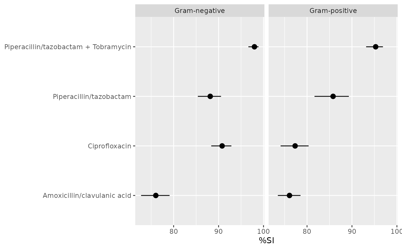
if (requireNamespace("ggplot2")) {
ggplot2::autoplot(ab1)
}
 if (requireNamespace("ggplot2")) {
ggplot2::autoplot(ab2)
}
if (requireNamespace("ggplot2")) {
ggplot2::autoplot(ab2)
}
 plot(ab1)
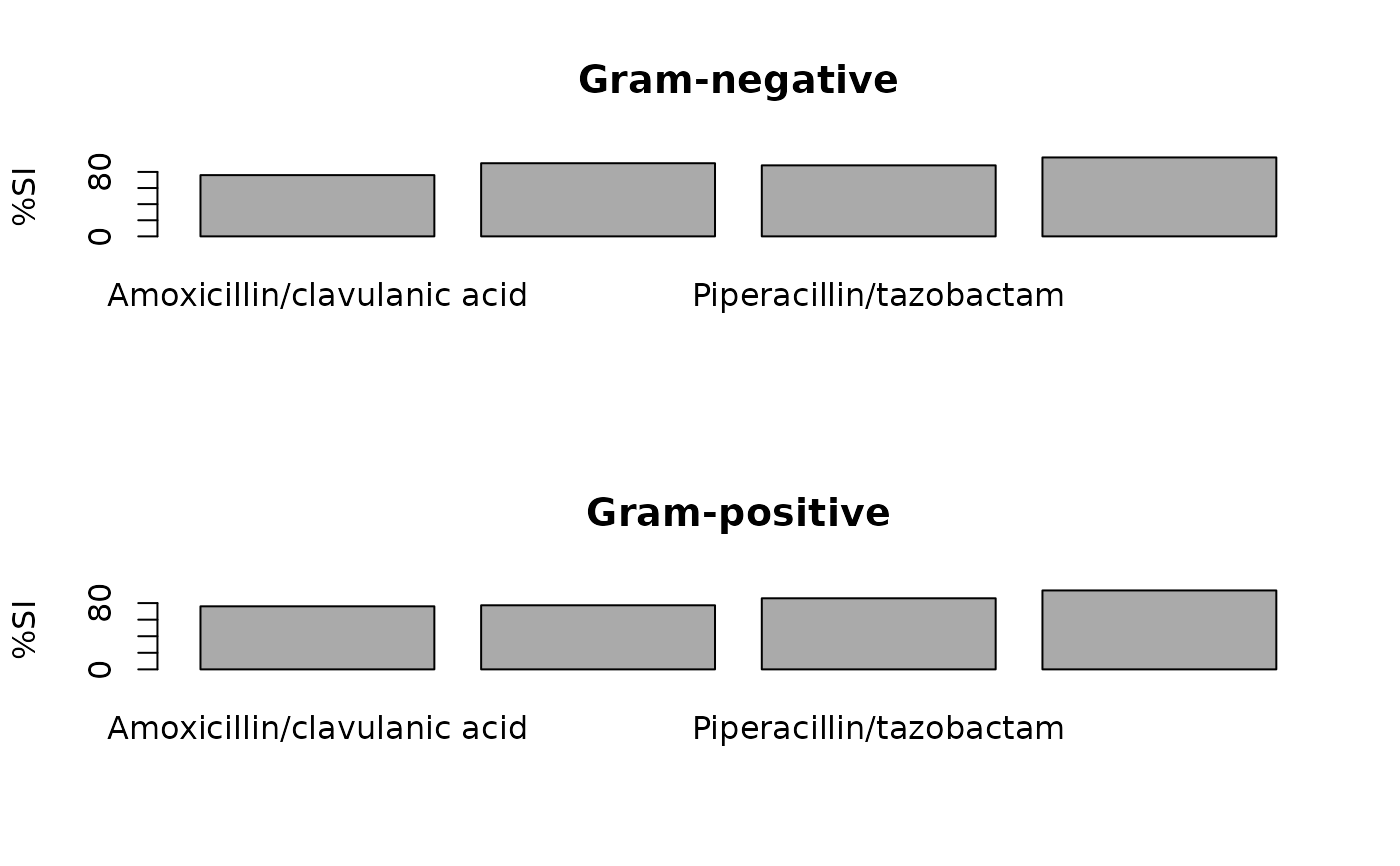 plot(ab2)
 # }
# }