19 KiB
Executable File
AMR
An R package to simplify the analysis and prediction of Antimicrobial Resistance (AMR) and work with antibiotic properties by using evidence-based methods.
This R package was created for academic research by PhD students of the Faculty of Medical Sciences of the University of Groningen and the Medical Microbiology & Infection Prevention (MMBI) department of the University Medical Center Groningen (UMCG).
▶️ Get it with install.packages("AMR") or see below for other possibilities. Read all changes and new functions in NEWS.md.
Authors
 Matthijs S. Berends1,2,a,
Christian F. Luz1,a,
Erwin E.A. Hassing2,
Corinna Glasner1,b,
Alex W. Friedrich1,b,
Bhanu Sinha1,b
Matthijs S. Berends1,2,a,
Christian F. Luz1,a,
Erwin E.A. Hassing2,
Corinna Glasner1,b,
Alex W. Friedrich1,b,
Bhanu Sinha1,b
1 Department of Medical Microbiology, University of Groningen, University Medical Center Groningen, Groningen, the Netherlands - rug.nl umcg.nl
2 Certe Medical Diagnostics & Advice, Groningen, the Netherlands - certe.nl
a R package author and thesis dissertant
b Thesis advisor
![]()
![]()
![]()
![]()
![]()
Contents
Why this package?
This R package was intended to make microbial epidemiology easier. Most functions contain extensive help pages to get started.
This AMR package basically does four important things:
-
It cleanses existing data, by transforming it to reproducible and profound classes, making the most efficient use of R. These function all use artificial intelligence to get expected results:
- Use
as.bactidto get an ID of a microorganism. It takes almost any text as input that looks like the name or code of a microorganism like "E. coli", "esco" and "esccol". Moreover, it can group all coagulase negative and positive Staphylococci, and can transform Streptococci into Lancefield groups. This package has a database of ~2500 different (potential) human pathogenic microorganisms. - Use
as.rsito transform values to valid antimicrobial results. It produces just S, I or R based on your input and warns about invalid values. Even values like "<=0.002; S" (combined MIC/RSI) will result in "S". - Use
as.micto cleanse your MIC values. It produces a so-called factor (in SPSS calls this ordinal) with valid MIC values as levels. A value like "<=0.002; S" (combined MIC/RSI) will result in "<=0.002". - Use
as.atcto get the ATC code of an antibiotic as defined by the WHO. This package contains a database with most LIS codes, official names, DDDs and even trade names of antibiotics. For example, the values "Furabid", "Furadantine", "nitro" will return the ATC code of Nitrofurantoine.
- Use
-
It enhances existing data and adds new data from data sets included in this package.
- Use
EUCAST_rulesto apply EUCAST expert rules to isolates. - Use
MDRO(abbreviation of Multi Drug Resistant Organisms) to check your isolates for exceptional resistance with country-specific guidelines with or EUCAST rules. Currently, national guidelines for Germany and the Netherlands are supported. - Data set
microorganismscontains the family, genus, species, subspecies, colloqual name and Gram stain of almost 2500 microorganisms. This enables e.g. resistance analysis of different antibiotics per Gram stain. - Data set
antibioticscontains the ATC code, LIS codes, official name, trivial name, trade name and DDD of both oral and parenteral administration. - Use
first_isolateto identify the first isolates of every patient using guidelines from the CLSI (Clinical and Laboratory Standards Institute). * You can also identify first weighted isolates of every patient, an adjusted version of the CLSI guideline. This takes into account key antibiotics of every strain and compares them.
- Use
-
It analyses the data with convenient functions that use well-known methods.
- Calculate the resistance (and even co-resistance) of microbial isolates with the
portion_R,portion_IR,portion_I,portion_SIandportion_Sfunctions, that can also be used with thedplyrpackage (e.g. in conjunction withsummarise) - Plot AMR results with
geom_rsi, a function made for theggplot2package - Predict antimicrobial resistance for the nextcoming years using logistic regression models with the
resistance_predictfunction - Conduct descriptive statistics to enhance base R: calculate kurtosis, skewness and create frequency tables
- Calculate the resistance (and even co-resistance) of microbial isolates with the
-
It teaches the user how to use all the above actions, by showing many examples in the help pages. The package contains an example data set called
septic_patients. This data set, consisting of 2000 blood culture isolates from anonymised septic patients between 2001 and 2017 in the Northern Netherlands, is real and genuine data.
How to get it?
All versions of this package are published on CRAN, the official R network with a peer-reviewed submission process.
Install from CRAN
(Note: Downloads measured only by cran.rstudio.com, this excludes e.g. the official cran.r-project.org)
-
Install using RStudio (recommended):
- Click on
Toolsand thenInstall Packages... - Type in
AMRand press Install
- Click on
-
Install in R directly:
install.packages("AMR")
Install from GitHub
This is the latest development version. Although it may contain bugfixes and even new functions compared to the latest released version on CRAN, it is also subject to change and may be unstable or behave unexpectedly. Always consider this a beta version.


![]()
install.packages("devtools")
devtools::install_github("msberends/AMR")
Install from Zenodo
![]()
This package was also published on Zenodo: https://doi.org/10.5281/zenodo.1305355
How to use it?
# Call it with:
library(AMR)

# For a list of functions:
help(package = "AMR")
New classes
This package contains two new S3 classes: mic for MIC values (e.g. from Vitek or Phoenix) and rsi for antimicrobial drug interpretations (i.e. S, I and R). Both are actually ordered factors under the hood (an MIC of 2 being higher than <=1 but lower than >=32, and for class rsi factors are ordered as S < I < R).
Both classes have extensions for existing generic functions like print, summary and plot.
These functions also try to coerce valid values.
RSI
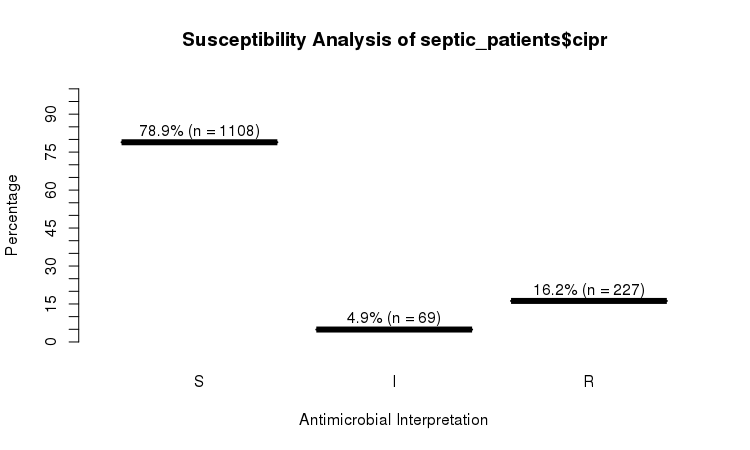
The septic_patients data set comes with antimicrobial results of more than 40 different drugs. For example, columns amox and cipr contain results of amoxicillin and ciprofloxacin, respectively.
summary(septic_patients[, c("amox", "cipr")])
#      amox          cipr
#  Mode  :rsi    Mode  :rsi
#  <NA>  :1002   <NA>  :596
#  Sum S :336    Sum S :1108
#  Sum IR:662    Sum IR:296
#  -Sum R:659    -Sum R:227
#  -Sum I:3      -Sum I:69
You can use the plot function from base R:
plot(septic_patients$cipr)
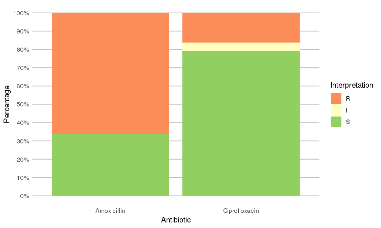
Or use the ggplot2 and dplyr packages to create more appealing plots:
library(dplyr)
library(ggplot2)

septic_patients %>%
  select(amox, cipr) %>%
  ggplot_rsi()
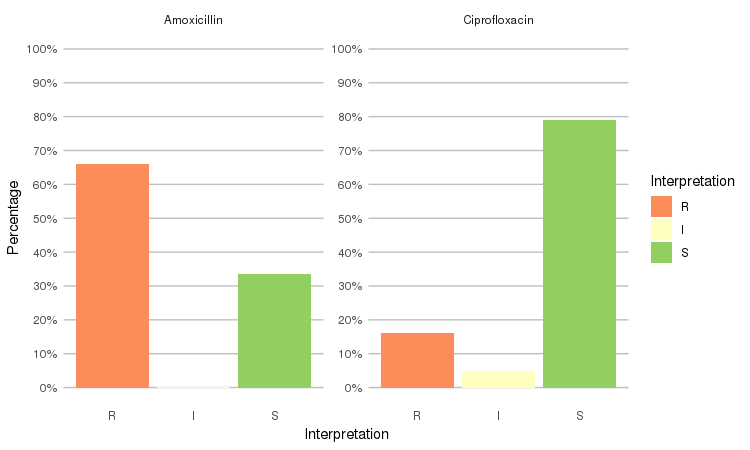
septic_patients %>%
    select(amox, cipr) %>%
    ggplot_rsi(x = "Interpretation", facet = "Antibiotic")
It also supports grouping variables. Let's say we want to compare resistance of drugs against Urine Tract Infections (UTI) between hospitals A to D (variable hospital_id):
septic_patients %>%
  select(hospital_id, amox, nitr, fosf, trim, cipr) %>%
  group_by(hospital_id) %>%
  ggplot_rsi(x = "hospital_id",
             facet = "Antibiotic",
             nrow = 1) +
  labs(title = "AMR of Anti-UTI Drugs Per Hospital",
       x = "Hospital")
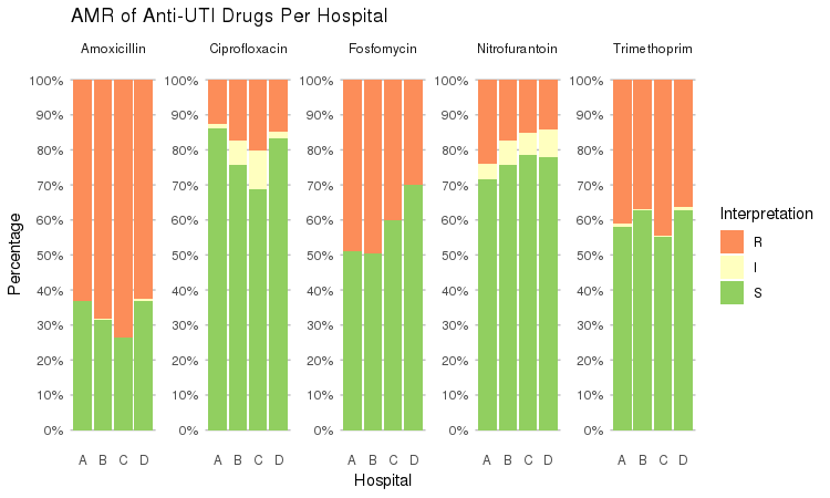
You could use this to group on anything in your plots: Gram stain, age (group), genus, geographic location, et cetera.
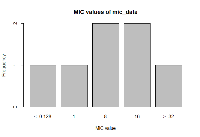
MIC
# Transform values to new class
mic_data <- as.mic(c(">=32", "1.0", "8", "<=0.128", "8", "16", "16"))

summary(mic_data)
#  Mode:mic
#  <NA>:0
#  Min.:<=0.128
#  Max.:>=32

plot(mic_data)
Overwrite/force resistance based on EUCAST rules
This is also called interpretive reading.
before <- data.frame(bactid = c("STAAUR",  # Staphylococcus aureus
                                "ENCFAE",  # Enterococcus faecalis
                                "ESCCOL",  # Escherichia coli
                                "KLEPNE",  # Klebsiella pneumoniae
                                "PSEAER"), # Pseudomonas aeruginosa
                     vanc = "-",           # Vancomycin
                     amox = "-",           # Amoxicillin
                     coli = "-",           # Colistin
                     cfta = "-",           # Ceftazidime
                     cfur = "-",           # Cefuroxime
                     stringsAsFactors = FALSE)
before
#   bactid vanc amox coli cfta cfur
# 1 STAAUR    -    -    -    -    -
# 2 ENCFAE    -    -    -    -    -
# 3 ESCCOL    -    -    -    -    -
# 4 KLEPNE    -    -    -    -    -
# 5 PSEAER    -    -    -    -    -

# Now apply those rules; just need a column with bacteria ID's and antibiotic results:
after <- EUCAST_rules(before)
after
#   bactid vanc amox coli cfta cfur
# 1 STAAUR    -    -    R    R    -
# 2 ENCFAE    -    -    R    R    R
# 3 ESCCOL    R    -    -    -    -
# 4 KLEPNE    R    R    -    -    -
# 5 PSEAER    R    R    -    -    R
Bacteria ID's can be retrieved with the guess_bactid function. It uses any type of info about a microorganism as input. For example, all these will return value STAAUR, the ID of S. aureus:
guess_bactid("stau")
guess_bactid("STAU")
guess_bactid("staaur")
guess_bactid("S. aureus")
guess_bactid("S aureus")
guess_bactid("Staphylococcus aureus")
guess_bactid("MRSA") # Methicillin Resistant S. aureus
guess_bactid("VISA") # Vancomycin Intermediate S. aureus
guess_bactid("VRSA") # Vancomycin Resistant S. aureus
Other (microbial) epidemiological functions
# G-test to replace Chi squared test
g.test(...)

# Determine key antibiotic based on bacteria ID
key_antibiotics(...)

# Selection of first isolates of any patient
first_isolate(...)

# Calculate resistance levels of antibiotics, can be used with `summarise` (dplyr)
rsi(...)
# Predict resistance levels of antibiotics
rsi_predict(...)

# Get name of antibiotic by ATC code
abname(...)
abname("J01CR02", from = "atc", to = "umcg") # "AMCL"
Frequency tables
Base R lacks a simple function to create frequency tables. We created such a function that works with almost all data types: freq (or frequency_tbl). It can be used in two ways:
# Like base R:
freq(mydata$myvariable)

# And like tidyverse:
mydata %>% freq(myvariable)
Factors sort on item by default:
septic_patients %>% freq(hospital_id)
# Frequency table of `hospital_id`
# Class:     factor
# Length:    2000 (of which NA: 0 = 0.0%)
# Unique:    4
#
#      Item    Count   Percent   Cum. Count   Cum. Percent   (Factor Level)
# ---  -----  ------  --------  -----------  -------------  ---------------
# 1    A         319     16.0%          319          16.0%                1
# 2    B         661     33.1%          980          49.0%                2
# 3    C         256     12.8%         1236          61.8%                3
# 4    D         764     38.2%         2000         100.0%                4
This can be changed with the sort.count parameter:
septic_patients %>% freq(hospital_id, sort.count = TRUE)
# Frequency table of `hospital_id`
# Class:     factor
# Length:    2000 (of which NA: 0 = 0.0%)
# Unique:    4
#
#      Item    Count   Percent   Cum. Count   Cum. Percent   (Factor Level)
# ---  -----  ------  --------  -----------  -------------  ---------------
# 1    D         764     38.2%          764          38.2%                4
# 2    B         661     33.1%         1425          71.2%                2
# 3    A         319     16.0%         1744          87.2%                1
# 4    C         256     12.8%         2000         100.0%                3
All other types, like numbers, characters and dates, sort on count by default:
septic_patients %>% freq(date)
# Frequency table of `date`
# Class:     Date
# Length:    2000 (of which NA: 0 = 0.0%)
# Unique:    1151
#
# Oldest:    2 January 2002
# Newest:    28 December 2017 (+5839)
# Median:    7 Augustus 2009 (~48%)
#
#      Item          Count   Percent   Cum. Count   Cum. Percent
# ---  -----------  ------  --------  -----------  -------------
# 1    2016-05-21       10      0.5%           10           0.5%
# 2    2004-11-15        8      0.4%           18           0.9%
# 3    2013-07-29        8      0.4%           26           1.3%
# 4    2017-06-12        8      0.4%           34           1.7%
# 5    2015-11-19        7      0.4%           41           2.1%
# 6    2005-12-22        6      0.3%           47           2.4%
# 7    2015-10-12        6      0.3%           53           2.6%
# 8    2002-05-16        5      0.2%           58           2.9%
# 9    2004-02-02        5      0.2%           63           3.1%
# 10   2004-02-18        5      0.2%           68           3.4%
# 11   2005-08-16        5      0.2%           73           3.6%
# 12   2005-09-01        5      0.2%           78           3.9%
# 13   2006-06-29        5      0.2%           83           4.2%
# 14   2007-08-10        5      0.2%           88           4.4%
# 15   2008-08-29        5      0.2%           93           4.7%
# [ reached getOption("max.print.freq") -- omitted 1136 entries, n = 1907 (95.3%) ]
For numeric values, some extra descriptive statistics will be calculated:
freq(runif(n = 10, min = 1, max = 5))
# Frequency table
# Class:     numeric
# Length:    10 (of which NA: 0 = 0.0%)
# Unique:    10
#
# Mean:      3.4
# Std. dev.: 1.3 (CV: 0.38, MAD: 1.3)
# Five-Num:  1.6 | 2.0 | 3.9 | 4.7 | 4.8 (IQR: 2.7, CQV: 0.4)
# Outliers:  0
#
#           Item   Count   Percent   Cum. Count   Cum. Percent
# ---  ---------  ------  --------  -----------  -------------
# 1     1.568997       1     10.0%            1          10.0%
# 2     1.993575       1     10.0%            2          20.0%
# 3     2.022348       1     10.0%            3          30.0%
# 4     2.236038       1     10.0%            4          40.0%
# 5     3.579828       1     10.0%            5          50.0%
# 6     4.178081       1     10.0%            6          60.0%
# 7     4.394818       1     10.0%            7          70.0%
# 8     4.689871       1     10.0%            8          80.0%
# 9     4.698626       1     10.0%            9          90.0%
# 10    4.751488       1     10.0%           10         100.0%
#
# Warning message:
# All observations are unique.
Learn more about this function with:
?freq
Data sets included in package
Datasets to work with antibiotics and bacteria properties.
# Dataset with 2000 random blood culture isolates from anonymised
# septic patients between 2001 and 2017 in 5 Dutch hospitals
septic_patients   # A tibble: 2,000 x 49

# Dataset with ATC antibiotics codes, official names, trade names
# and DDD's (oral and parenteral)
antibiotics       # A tibble: 420 x 18

# Dataset with bacteria codes and properties like gram stain and
# aerobic/anaerobic
microorganisms    # A tibble: 2,453 x 12
Copyright

This R package is licensed under the GNU General Public License (GPL) v2.0. In a nutshell, this means that this package:
-
May be used for commercial purposes
-
May be used for private purposes
-
May not be used for patent purposes
-
May be modified, although:
- Modifications must be released under the same license when distributing the package
- Changes made to the code must be documented
-
May be distributed, although:
- Source code must be made available when the package is distributed
- A copy of the license and copyright notice must be included with the package.
-
Comes with a LIMITATION of liability
-
Comes with NO warranty