AMR 
An R package to simplify the analysis and prediction of Antimicrobial Resistance (AMR) and work with antibiotic properties by using evidence-based methods.
This R package was created for academic research by PhD students of the Faculty of Medical Sciences of the University of Groningen and the Medical Microbiology & Infection Prevention (MMBI) department of the University Medical Center Groningen (UMCG).
▶️ Get it with install.packages("AMR") or see below for other possibilities.
▶️ Read the changelog here.
Authors
Matthijs S. Berends 1,2,a,
Christian F. Luz
1,a,
Erwin E.A. Hassing2,
Corinna Glasner
1,b,
Alex W. Friedrich
1,b,
Bhanu Sinha
1,b
1 Department of Medical Microbiology, University of Groningen, University Medical Center Groningen, Groningen, the Netherlands - rug.nl umcg.nl
2 Certe Medical Diagnostics & Advice, Groningen, the Netherlands - certe.nl
a R package author and thesis dissertant
b Thesis advisor
Contents
Why this package?
This R package was intended to make microbial epidemiology easier. Most functions contain extensive help pages to get started.
The AMR package basically does four important things:
-
It cleanses existing data, by transforming it to reproducible and profound classes, making the most efficient use of R. These functions all use artificial intelligence to guess results that you would expect:
- Use
as.moto get an ID of a microorganism. The IDs are human readable for the trained eye - the ID of Klebsiella pneumoniae is "B_KLBSL_PNE" (B stands for Bacteria) and the ID of S. aureus is "B_STPHY_AUR". The function takes almost any text as input that looks like the name or code of a microorganism like "E. coli", "esco" and "esccol". Evenas.mo("MRSA")will return the ID of S. aureus. Moreover, it can group all coagulase negative and positive Staphylococci, and can transform Streptococci into Lancefield groups. To find bacteria based on your input, it uses Artificial Intelligence to look up values in the included ITIS data, consisting of more than 18,000 microorganisms. - Use
as.rsito transform values to valid antimicrobial results. It produces just S, I or R based on your input and warns about invalid values. Even values like "<=0.002; S" (combined MIC/RSI) will result in "S". - Use
as.micto cleanse your MIC values. It produces a so-called factor (called ordinal in SPSS) with valid MIC values as levels. A value like "<=0.002; S" (combined MIC/RSI) will result in "<=0.002". - Use
as.atcto get the ATC code of an antibiotic as defined by the WHO. This package contains a database with most LIS codes, official names, DDDs and even trade names of antibiotics. For example, the values "Furabid", "Furadantin", "nitro" all return the ATC code of Nitrofurantoine.
- Use
-
It enhances existing data and adds new data from data sets included in this package.
- Use
EUCAST_rulesto apply EUCAST expert rules to isolates. - Use
first_isolateto identify the first isolates of every patient using guidelines from the CLSI (Clinical and Laboratory Standards Institute).- You can also identify first weighted isolates of every patient, an adjusted version of the CLSI guideline. This takes into account key antibiotics of every strain and compares them.
- Use
MDRO(abbreviation of Multi Drug Resistant Organisms) to check your isolates for exceptional resistance with country-specific guidelines or EUCAST rules. Currently, national guidelines for Germany and the Netherlands are supported. - The data set
microorganismscontains the complete taxonomic tree of more than 18,000 microorganisms (bacteria, fungi/yeasts and protozoa). Furthermore, the colloquial name and Gram stain are available, which enables resistance analysis of e.g. different antibiotics per Gram stain. The package also contains functions to look up values in this data set likemo_genus,mo_family,mo_gramstainor evenmo_phylum. As they useas.mointernally, they also use artificial intelligence. For example,mo_genus("MRSA")andmo_genus("S. aureus")will both return"Staphylococcus". They also come with support for German, Dutch, French, Italian, Spanish and Portuguese. These functions can be used to add new variables to your data. - The data set
antibioticscontains the ATC code, LIS codes, official name, trivial name and DDD of both oral and parenteral administration. It also contains a total of 298 trade names. Use functions likeab_nameandab_tradenamesto look up values. Theab_*functions useas.atcinternally so they support AI to guess your expected result. For example,ab_name("Fluclox"),ab_name("Floxapen")andab_name("J01CF05")will all return"Flucloxacillin". These functions can again be used to add new variables to your data.
- Use
-
It analyses the data with convenient functions that use well-known methods.
- Calculate the resistance (and even co-resistance) of microbial isolates with the
portion_R,portion_IR,portion_I,portion_SIandportion_Sfunctions. Similarly, the amount of isolates can be determined with thecount_R,count_IR,count_I,count_SIandcount_Sfunctions. All these functions can be used with thedplyrpackage (e.g. in conjunction withsummarise) - Plot AMR results with
geom_rsi, a function made for theggplot2package - Predict antimicrobial resistance for the nextcoming years using logistic regression models with the
resistance_predictfunction - Conduct descriptive statistics to enhance base R: calculate kurtosis, skewness and create frequency tables
- Calculate the resistance (and even co-resistance) of microbial isolates with the
-
It teaches the user how to use all the above actions.
- The package contains extensive help pages with many examples.
- It also contains an example data set called
septic_patients. This data set contains:- 2,000 blood culture isolates from anonymised septic patients between 2001 and 2017 in the Northern Netherlands
- Results of 40 antibiotics (each antibiotic in its own column) with a total of 38,414 antimicrobial results
- Real and genuine data
ITIS

This package contains the complete microbial taxonomic data (with all seven taxonomic ranks - from subkingdom to subspecies) from the publicly available Integrated Taxonomic Information System (ITIS, https://www.itis.gov).
All (sub)species from the taxonomic kingdoms Bacteria, Fungi and Protozoa are included in this package, as well as all previously accepted names known to ITIS. Furthermore, the responsible authors and year of publication are available. This allows users to use authoritative taxonomic information for their data analysis on any microorganism, not only human pathogens.
ITIS is a partnership of U.S., Canadian, and Mexican agencies and taxonomic specialists.
Get a note when a species was renamed
mo_shortname("Chlamydia psittaci")
# Note: 'Chlamydia psittaci' (Page, 1968) was renamed 'Chlamydophila psittaci' (Everett et al., 1999)
# [1] "C. psittaci"
Get any property from the entire taxonomic tree for all included species
mo_class("E. coli")
# [1] "Gammaproteobacteria"

mo_family("E. coli")
# [1] "Enterobacteriaceae"

mo_ref("E. coli")
# [1] "Castellani and Chalmers, 1919"
Do not get mistaken - the package only includes microorganisms
mo_phylum("C. elegans")
# [1] "Cyanobacteria"                   # Bacteria?!
mo_fullname("C. elegans")
# [1] "Chroococcus limneticus elegans"  # Because a microorganism was found
How to get it?
All stable versions of this package are published on CRAN, the official R network with a peer-reviewed submission process.
Install from CRAN
(Note: Downloads measured only by cran.rstudio.com, this excludes e.g. the official cran.r-project.org)
-
Install using RStudio (recommended):
- Click on
Toolsand thenInstall Packages... - Type in
AMRand press Install
- Click on
-
install.packages("AMR")
Install from Zenodo
This package was also published on Zenodo (stable releases only): https://doi.org/10.5281/zenodo.1305355
Install from GitLab
This is the latest development version. Although it may contain bugfixes and even new functions compared to the latest released version on CRAN, it is also subject to change and may be unstable or behave unexpectedly. Always consider this a beta version. All below 'badges' should be green:
| Development Test | Result | Reference |
|---|---|---|
| All functions checked on Linux and macOS | GitLab [ref 1] | |
| All functions checked on Windows | Appveyor Systems Inc. [ref 2] | |
| Percentage of syntax lines checked | Codecov LLC [ref 3] |
If so, try it with:
install.packages("devtools")
devtools::install_git("https://gitlab.com/msberends/AMR")
How to use it?
# Call it with:
library(AMR)

# For a list of functions:
help(package = "AMR")
New classes
This package contains two new S3 classes: mic for MIC values (e.g. from Vitek or Phoenix) and rsi for antimicrobial drug interpretations (i.e. S, I and R). Both are actually ordered factors under the hood (an MIC of 2 being higher than <=1 but lower than >=32, and for class rsi factors are ordered as S < I < R).
Both classes have extensions for existing generic functions like print, summary and plot.
These functions also try to coerce valid values.
RSI
The septic_patients data set comes with antimicrobial results of more than 40 different drugs. For example, columns amox and cipr contain results of amoxicillin and ciprofloxacin, respectively.
summary(septic_patients[, c("amox", "cipr")])
#      amox          cipr
#  Mode  :rsi    Mode  :rsi
#  <NA>  :1002   <NA>  :596
#  Sum S :336    Sum S :1108
#  Sum IR:662    Sum IR:296
#  -Sum R:659    -Sum R:227
#  -Sum I:3      -Sum I:69
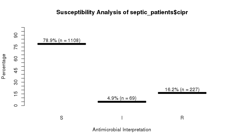
You can use the plot function from base R:
plot(septic_patients$cipr)
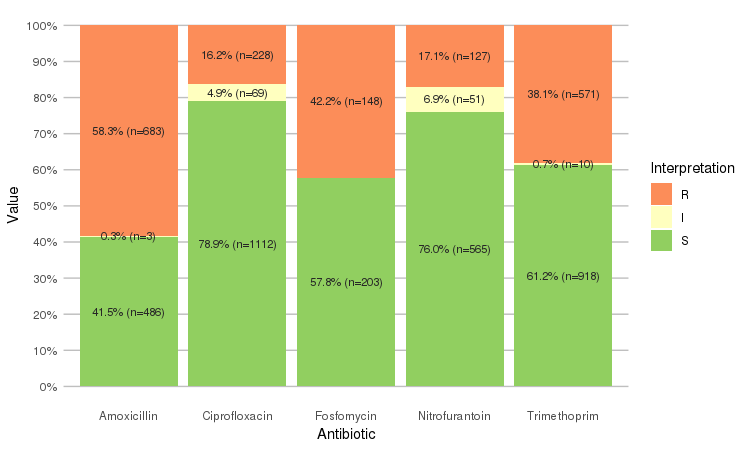
Or use the ggplot2 and dplyr packages to create more appealing plots:
library(dplyr)
library(ggplot2)

septic_patients %>%
  select(amox, nitr, fosf, trim, cipr) %>%
  ggplot_rsi()
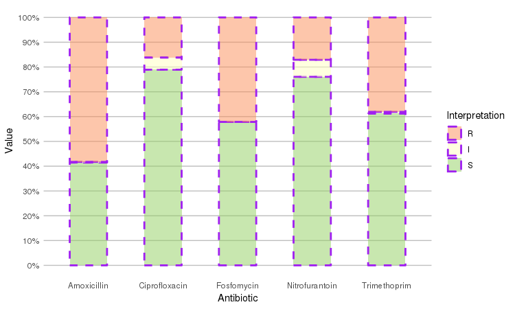
Adjust it with any parameter you know from the ggplot2 package:
septic_patients %>%
  select(amox, nitr, fosf, trim, cipr) %>%
  ggplot_rsi(datalabels = FALSE,
             width = 0.5, colour = "purple", size = 1, linetype = 2, alpha = 0.5)
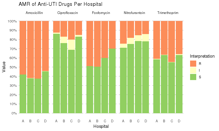
It also supports grouping variables. Let's say we want to compare resistance of drugs against Urine Tract Infections (UTI) between hospitals A to D (variable hospital_id):
septic_patients %>%
  select(hospital_id, amox, nitr, fosf, trim, cipr) %>%
  group_by(hospital_id) %>%
  ggplot_rsi(x = "hospital_id",
             facet = "Antibiotic",
             nrow = 1,
             datalabels = FALSE) +
  labs(title = "AMR of Anti-UTI Drugs Per Hospital",
       x = "Hospital")
You could use this to group on anything in your plots: Gram stain, age (group), genus, geographic location, et cetera.
Is there a significant difference between hospital A and D when it comes to Fosfomycin?
check_A_and_D <- septic_patients %>%
  filter(hospital_id %in% c("A", "D")) %>% # filter on only hospitals A and D
  select(hospital_id, fosf) %>%            # select the hospitals and fosfomycin
  group_by(hospital_id) %>%
  count_df(combine_IR = TRUE) %>%          # count all isolates per group (hospital_id)
  tidyr::spread(hospital_id, Value) %>%    # transform output so A and D are columns
  select(A, D) %>%                         # and select these only
  as.matrix()                              # transform to good old matrix for fisher.test

check_A_and_D
#       A  D
# [1,] 24 33
# [2,] 25 77
Total sum is lower than 1,000 so we'd prefer a Fisher's exact test, not a G-test (or its formerly used equivalent, the famous Chi2 test):
fisher.test(check_A_and_D)
#
# 	Fisher's Exact Test for Count Data
#
# data:  check_A_and_D
# p-value = 0.03104
# alternative hypothesis: true odds ratio is not equal to 1
# 95 percent confidence interval:
#  1.054283 4.735995
# sample estimates:
# odds ratio
#   2.228006
Well, there you go!
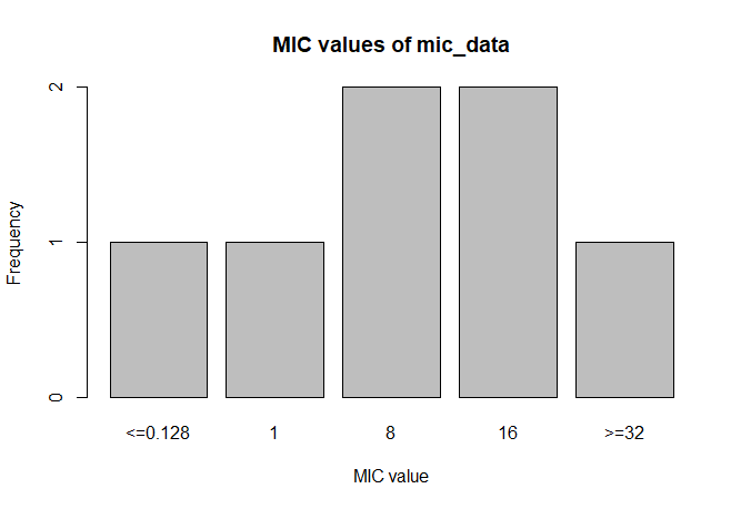
MIC
# Transform values to new class
mic_data <- as.mic(c(">=32", "1.0", "8", "<=0.128", "8", "16", "16"))

summary(mic_data)
#  Mode:mic
#  <NA>:0
#  Min.:<=0.128
#  Max.:>=32

plot(mic_data)
Overwrite/force resistance based on EUCAST rules
This is also called interpretive reading.
a <- data.frame(mo = c("Staphylococcus aureus",
                       "Enterococcus faecalis",
                       "Escherichia coli",
                       "Klebsiella pneumoniae",
                       "Pseudomonas aeruginosa"),
                vanc = "-",       # Vancomycin
                amox = "-",       # Amoxicillin
                coli = "-",       # Colistin
                cfta = "-",       # Ceftazidime
                cfur = "-",       # Cefuroxime
                peni = "S",       # Benzylpenicillin
                cfox = "S",       # Cefoxitin
                stringsAsFactors = FALSE)

a
#                       mo vanc amox coli cfta cfur peni cfox
# 1  Staphylococcus aureus    -    -    -    -    -    S    S
# 2  Enterococcus faecalis    -    -    -    -    -    S    S
# 3       Escherichia coli    -    -    -    -    -    S    S
# 4  Klebsiella pneumoniae    -    -    -    -    -    S    S
# 5 Pseudomonas aeruginosa    -    -    -    -    -    S    S

b <- EUCAST_rules(a) # 18 results are forced as R or S

b
#                       mo vanc amox coli cfta cfur peni cfox
# 1  Staphylococcus aureus    -    S    R    R    S    S    S
# 2  Enterococcus faecalis    -    -    R    R    R    S    R
# 3       Escherichia coli    R    -    -    -    -    R    S
# 4  Klebsiella pneumoniae    R    R    -    -    -    R    S
# 5 Pseudomonas aeruginosa    R    R    -    -    R    R    R
Bacteria IDs can be retrieved with the guess_mo function. It uses any type of info about a microorganism as input. For example, all these will return value B_STPHY_AUR, the ID of S. aureus:
guess_mo("stau")
guess_mo("STAU")
guess_mo("staaur")
guess_mo("S. aureus")
guess_mo("S aureus")
guess_mo("Staphylococcus aureus")
guess_mo("MRSA") # Methicillin Resistant S. aureus
guess_mo("MSSA") # Methicillin Susceptible S. aureus
guess_mo("VISA") # Vancomycin Intermediate S. aureus
guess_mo("VRSA") # Vancomycin Resistant S. aureus
Other (microbial) epidemiological functions
# G-test to replace Chi squared test
g.test(...)

# Determine key antibiotic based on bacteria ID
key_antibiotics(...)

# Selection of first isolates of any patient
first_isolate(...)

# Calculate resistance levels of antibiotics, can be used with `summarise` (dplyr)
rsi(...)
# Predict resistance levels of antibiotics
rsi_predict(...)

# Get name of antibiotic by ATC code
abname(...)
abname("J01CR02", from = "atc", to = "umcg") # "AMCL"
Frequency tables
Base R lacks a simple function to create frequency tables. We created such a function that works with almost all data types: freq (or frequency_tbl). It can be used in two ways:
# Like base R:
freq(mydata$myvariable)

# And like tidyverse:
mydata %>% freq(myvariable)
Frequency are of course sorted by count at default:
septic_patients %>% freq(hospital_id)
# Class:     factor (numeric)
# Length:    2000 (of which NA: 0 = 0.00%)
# Unique:    4
#
#      Item    Count   Percent   Cum. Count   Cum. Percent
# ---  -----  ------  --------  -----------  -------------
# 1    D         762     38.1%          762          38.1%
# 2    B         663     33.1%         1425          71.2%
# 3    A         321     16.1%         1746          87.3%
# 4    C         254     12.7%         2000         100.0%
This can be changed with the sort.count parameter:
septic_patients %>% freq(hospital_id, sort.count = FALSE)
# Class:     factor (numeric)
# Length:    2000 (of which NA: 0 = 0.00%)
# Unique:    4
#
#      Item    Count   Percent   Cum. Count   Cum. Percent
# ---  -----  ------  --------  -----------  -------------
# 1    A         321     16.1%          321          16.1%
# 2    B         663     33.1%          984          49.2%
# 3    C         254     12.7%         1238          61.9%
# 4    D         762     38.1%         2000         100.0%
For numeric values, some extra descriptive statistics will be calculated:
freq(runif(n = 10, min = 1, max = 5))
# Frequency table
# Class:     numeric
# Length:    10 (of which NA: 0 = 0.00%)
# Unique:    10
#
# Mean:      3.1
# Std. dev.: 1.3 (CV: 0.43, MAD: 1.8)
# Five-Num:  1.3 | 1.7 | 3.2 | 4.3 | 5.0 (IQR: 2.6, CQV: 0.43)
# Outliers:  0
#
#           Item   Count   Percent   Cum. Count   Cum. Percent
# ---  ---------  ------  --------  -----------  -------------
# 1     1.271079       1     10.0%            1          10.0%
# 2     1.333975       1     10.0%            2          20.0%
# 3     1.714946       1     10.0%            3          30.0%
# 4     2.751871       1     10.0%            4          40.0%
# 5     3.090140       1     10.0%            5          50.0%
# 6     3.260850       1     10.0%            6          60.0%
# 7     3.824105       1     10.0%            7          70.0%
# 8     4.278028       1     10.0%            8          80.0%
# 9     4.436265       1     10.0%            9          90.0%
# 10    4.996694       1     10.0%           10         100.0%
#
# Warning message:
# All observations are unique.
Learn more about this function with:
?freq
Data sets included in package
Data sets to work with antibiotics and bacteria properties.
# Data set with complete taxonomic trees from ITIS, containing of
# the three kingdoms Bacteria, Fungi and Protozoa
microorganisms     # data.frame: 18,833 x 15
microorganisms.old # data.frame: 2,383 x 4

# Data set with ATC antibiotics codes, official names, trade names
# and DDDs (oral and parenteral)
antibiotics       #  data.frame: 423 x 18

# Data set with 2000 random blood culture isolates from anonymised
# septic patients between 2001 and 2017 in 5 Dutch hospitals
septic_patients    # data.frame: 2,000 x 49
Benchmarks
One of the most important features of this package is the complete microbial taxonomic database, supplied by ITIS (https://www.itis.gov). We created a function as.mo that transforms any user input value to a valid microbial ID by using AI (Artificial Intelligence) and based on the taxonomic tree of ITIS.
Using the microbenchmark package, we can review the calculation performance of this function.
library(microbenchmark)
In the next test, we try to 'coerce' different input values for Staphylococcus aureus. The actual result is the same every time: it returns its MO code B_STAPHY_AUR (B stands for Bacteria, the taxonomic kingdom).
But the calculation time differs a lot. Here, the AI effect can be reviewed best:
microbenchmark(A = as.mo("stau"),
               B = as.mo("staaur"),
               C = as.mo("S. aureus"),
               D = as.mo("S.  aureus"),
               E = as.mo("STAAUR"),
               F = as.mo("Staphylococcus aureus"),
               times = 10,
               unit = "ms")
# Unit: milliseconds
#  expr      min       lq     mean   median       uq      max neval
#     A 36.05088 36.14782 36.65635 36.24466 36.43075 39.78544    10
#     B 16.43575 16.46885 16.67816 16.66053 16.84858 16.95299    10
#     C 14.44150 14.52182 16.81197 14.59173 14.67854 36.75244    10
#     D 14.49765 14.58153 16.71666 14.59414 14.61094 35.50731    10
#     E 14.45212 14.75146 14.82033 14.85559 14.96433 15.03438    10
#     F 10.69445 10.73852 10.80334 10.79596 10.86856 10.97465    10
The more an input value resembles a full name, the faster the result will be found. In the table above, all measurements are in milliseconds, tested on a quite regular Linux server from 2007 with 2 GB RAM. A value of 10.8 milliseconds means it will roughly determine 93 different (unique) input values per second. It case of 36.2 milliseconds, this is only 28 input values per second.
To improve speed, the as.mo function also takes into account the prevalence of human pathogenic microorganisms. The downside is of course that less prevalent microorganisms will be determined far less faster. See this example for the ID of Burkholderia nodosa (B_BRKHL_NOD):
microbenchmark(B = as.mo("burnod"),
               C = as.mo("B. nodosa"),
               D = as.mo("B.  nodosa"),
               E = as.mo("BURNOD"),
               F = as.mo("Burkholderia nodosa"),
               times = 10,
               unit = "ms")
# Unit: milliseconds
#  expr      min        lq      mean    median        uq       max neval
#     B 175.9446 176.80440 179.18240 177.00131 177.62021 198.86286    10
#     C  88.1902  88.57705  89.08851  88.84293  89.15498  91.76621    10
#     D 110.2641 110.67497 113.66290 111.20534 111.80744 134.44699    10
#     E 175.0728 177.04235 207.83542 190.38109 200.33448 388.12177    10
#     F  45.0778  45.31617  52.72430  45.62962  67.85262  70.42250    10
(Note: A is missing here, because as.mo("buno") returns F_BUELL_NOT: the ID of the fungus Buellia notabilis)
That takes up to 12 times as much time! A value of 190.4 milliseconds means it can only determine ~5 different input values per second. We can conclude that looking up arbitrary codes of less prevalent microorganisms is the worst way to go, in terms of calculation performance.
To relieve this pitfall and further improve performance, two important calculations take almost no time at all: repetive results and already precalculated results.
Let's set up 25,000 entries of "Staphylococcus aureus" and check its speed:
repetive_results <- rep("Staphylococcus aureus", 25000)
microbenchmark(A = as.mo(repetive_results),
               times = 10,
               unit = "ms")
# Unit: milliseconds
#  expr      min       lq     mean   median       uq      max neval
#     A 14.61282  14.6372 14.70817 14.72597 14.76124 14.78498    10
So transforming 25,000 times (!) "Staphylococcus aureus" only takes 4 ms (0.004 seconds) more than transforming it once. You only lose time on your unique input values.
What about precalculated results? This package also contains helper functions for specific microbial properties, for example mo_fullname. It returns the full microbial name (genus, species and possibly subspecies) and uses as.mo internally. If the input is however an already precalculated result, it almost doesn't take any time at all (see 'C' below):
microbenchmark(A = mo_fullname("B_STPHY_AUR"),
               B = mo_fullname("S. aureus"),
               C = mo_fullname("Staphylococcus aureus"),
               times = 10,
               unit = "ms")
# Unit: milliseconds
#  expr       min       lq       mean    median        uq       max neval
#     A 13.548652 13.74588 13.8052969 13.813594 13.881165 14.090969    10
#     B 15.079781 15.16785 15.3835842 15.374477 15.395115 16.072995    10
#     C  0.171182  0.18563  0.2306307  0.203413  0.224610  0.492312    10
So going from mo_fullname("Staphylococcus aureus") to "Staphylococcus aureus" takes 0.0002 seconds - it doesn't even start calculating if the result would be the same as the expected resulting value. That goes for all helper functions:
microbenchmark(A = mo_species("aureus"),
               B = mo_genus("Staphylococcus"),
               C = mo_fullname("Staphylococcus aureus"),
               D = mo_family("Staphylococcaceae"),
               E = mo_order("Bacillales"),
               F = mo_class("Bacilli"),
               G = mo_phylum("Firmicutes"),
               H = mo_subkingdom("Posibacteria"),
               times = 10,
               unit = "ms")
# Unit: milliseconds
#  expr      min       lq      mean    median       uq      max neval
#     A 0.145270 0.158750 0.1908419 0.1693655 0.218255 0.300528    10
#     B 0.182985 0.184522 0.2025408 0.1970235 0.209944 0.243328    10
#     C 0.176280 0.201632 0.2618147 0.2303025 0.339499 0.388249    10
#     D 0.136890 0.139054 0.1552231 0.1518010 0.168738 0.193042    10
#     E 0.100921 0.116496 0.1321823 0.1222930 0.129976 0.230477    10
#     F 0.103017 0.110281 0.1214480 0.1199880 0.124319 0.147506    10
#     G 0.099246 0.110280 0.1195553 0.1188705 0.125436 0.149741    10
#     H 0.114331 0.117264 0.1249819 0.1220830 0.129557 0.143385    10
Of course, when running mo_phylum("Firmicutes") the function has zero knowledge about the actual microorganism, namely S. aureus. But since the result would be "Firmicutes" too, there is no point in calculating the result. And since this package 'knows' all phyla of all known microorganisms (according to ITIS), it can just return the initial value immediately.
Copyright
This R package is licensed under the GNU General Public License (GPL) v2.0. In a nutshell, this means that this package:
-
May be used for commercial purposes
-
May be used for private purposes
-
May not be used for patent purposes
-
May be modified, although:
- Modifications must be released under the same license when distributing the package
- Changes made to the code must be documented
-
May be distributed, although:
- Source code must be made available when the package is distributed
- A copy of the license and copyright notice must be included with the package.
-
Comes with a LIMITATION of liability
-
Comes with NO warranty


